Loading [MathJax]/jax/output/SVG/jax.js

Mean-field limit of collective dynamics with time-varying weights

  • Received: 01 April 2021 Revised: 01 October 2021 Published: 18 February 2022
  • Primary: 35Q70, 34A34; Secondary: 35L60

  • In this paper, we derive the mean-field limit of a collective dynamics model with time-varying weights, for weight dynamics that preserve the total mass of the system as well as indistinguishability of the agents. The limit equation is a transport equation with source, where the (non-local) transport term corresponds to the position dynamics, and the (non-local) source term comes from the weight redistribution among the agents. We show existence and uniqueness of the solution for both microscopic and macroscopic models and introduce a new empirical measure taking into account the weights. We obtain the convergence of the microscopic model to the macroscopic one by showing continuity of the macroscopic solution with respect to the initial data, in the Wasserstein and Bounded Lipschitz topologies.

    Citation: Nastassia Pouradier Duteil. Mean-field limit of collective dynamics with time-varying weights[J]. Networks and Heterogeneous Media, 2022, 17(2): 129-161. doi: 10.3934/nhm.2022001

    Related Papers:

    [1] Charles Bordenave, David R. McDonald, Alexandre Proutière . A particle system in interaction with a rapidly varying environment: Mean field limits and applications. Networks and Heterogeneous Media, 2010, 5(1): 31-62. doi: 10.3934/nhm.2010.5.31
    [2] Michele Gianfelice, Enza Orlandi . Dynamics and kinetic limit for a system of noiseless $d$-dimensional Vicsek-type particles. Networks and Heterogeneous Media, 2014, 9(2): 269-297. doi: 10.3934/nhm.2014.9.269
    [3] Fabio Camilli, Italo Capuzzo Dolcetta, Maurizio Falcone . Preface. Networks and Heterogeneous Media, 2012, 7(2): i-ii. doi: 10.3934/nhm.2012.7.2i
    [4] Peter V. Gordon, Cyrill B. Muratov . Self-similarity and long-time behavior of solutions of the diffusion equation with nonlinear absorption and a boundary source. Networks and Heterogeneous Media, 2012, 7(4): 767-780. doi: 10.3934/nhm.2012.7.767
    [5] Maria Teresa Chiri, Xiaoqian Gong, Benedetto Piccoli . Mean-field limit of a hybrid system for multi-lane car-truck traffic. Networks and Heterogeneous Media, 2023, 18(2): 723-752. doi: 10.3934/nhm.2023031
    [6] Olivier Guéant . New numerical methods for mean field games with quadratic costs. Networks and Heterogeneous Media, 2012, 7(2): 315-336. doi: 10.3934/nhm.2012.7.315
    [7] Michael Herty, Lorenzo Pareschi, Giuseppe Visconti . Mean field models for large data–clustering problems. Networks and Heterogeneous Media, 2020, 15(3): 463-487. doi: 10.3934/nhm.2020027
    [8] Michael Herty, Lorenzo Pareschi, Sonja Steffensen . Mean--field control and Riccati equations. Networks and Heterogeneous Media, 2015, 10(3): 699-715. doi: 10.3934/nhm.2015.10.699
    [9] Seung-Yeal Ha, Jeongho Kim, Jinyeong Park, Xiongtao Zhang . Uniform stability and mean-field limit for the augmented Kuramoto model. Networks and Heterogeneous Media, 2018, 13(2): 297-322. doi: 10.3934/nhm.2018013
    [10] Martino Bardi . Explicit solutions of some linear-quadratic mean field games. Networks and Heterogeneous Media, 2012, 7(2): 243-261. doi: 10.3934/nhm.2012.7.243
  • In this paper, we derive the mean-field limit of a collective dynamics model with time-varying weights, for weight dynamics that preserve the total mass of the system as well as indistinguishability of the agents. The limit equation is a transport equation with source, where the (non-local) transport term corresponds to the position dynamics, and the (non-local) source term comes from the weight redistribution among the agents. We show existence and uniqueness of the solution for both microscopic and macroscopic models and introduce a new empirical measure taking into account the weights. We obtain the convergence of the microscopic model to the macroscopic one by showing continuity of the macroscopic solution with respect to the initial data, in the Wasserstein and Bounded Lipschitz topologies.


    A wide range of mathematical models fall into the category of interacting particle systems. Whether they describe the trajectories of colliding particles [7], the behavior of animal groups [1,6,13,22], the cooperation of robots [4] or the evolution of opinions [9,12,15], their common objective is to model the dynamics of a group of particles in interaction. Some of the most widely used models include the Hegselmann-Krause model for opinion dynamics [15], the Vicsek model for fish behavior [22] and the Cucker-Smale model for bird flocks [6]. Two main points of view can be adopted in the modeling process. The Lagrangian (or microscopic) approach deals with individual particles and models the trajectory of each one separately, via a system of coupled Ordinary Differential Equations (ODE). This approach's major limitation is that the dimension of the resulting system is proportional to the number of particles, which can quickly become unmanageable. To combat this effect, one can instead adopt the Eulerian (or macroscopic) approach, and track the concentration of particles at each point of the state space. The resulting equation is a Partial Differential Equation (PDE) giving the evolution of the density of particles over the state space, and whose dimension is independent of the number of particles.

    The question of how microscopic properties of particles give rise to macroscopic properties of the system is fundamental in physics. A way to connect the microscopic and the macroscopic points of view is through the mean-field limit. First introduced in the context of gas dynamics, the mean-field limit, applied to systems of weakly interacting particles with a large radius of interaction, derives the macroscopic equation as the limit of the microscopic one when the number of particles tends to infinity [3,10]. The term mean-field refers to the fact that the effects of all particles located at the same position are averaged, instead of considering the individual force exerted by each particle. The mean-field limits of the Hegselmann-Krause, Vicsek and Cucker-Smale models were derived in [5,8,10,14]. More specifically, the mean-field limit of a general system of interacting particles described by

    ˙xi(t)=1NNj=1ϕ(xj(t)xi(t)) (1)

    is given by the non-local transport equation in the space of probability measures

    tμt(x)+(V[μt](x)μt(x))=0,V[μt](x)=Rdϕ(yx)dμt(y), (2)

    where μt(x) represents the density of particles at position x and time t, and where the velocity V[μt] is given by convolution with the density of particles. The proof of the mean-field limit lies on the key observation that the empirical measure μNt=1NNi=1δxi(t), defined from the positions of the N particles satisfying the microscopic system (1), is actually a solution to the macroscopic equation (2). Notice that the passage from the microscopic system to its macroscopic formulation via the empirical measure entails an irreversible information loss. Indeed, the empirical measure keeps track only of the number (or proportion) of particles at each point of space, and loses the information of the indices, that is the "identity" of the particles. This observation illustrates a necessary condition for the mean-field limit to hold: the indistinguishability of particles. Informally, two particles xi, xj are said to be indistinguishable if they can be exchanged without modifying the dynamics of the other particles. System (1) satisfies trivially this condition, since the interaction function ϕ depends only on the positions of the particles and not on their indices.

    In [16,17], we introduced an augmented model for opinion dynamics with time-varying influence. In this model, each particle, or agent, is represented both by its opinion xi and its weight of influence mi. The weights are assumed to evolve in time via their own dynamics, and model a modulating social hierarchy within the group, where the most influential agents (the ones with the largest weights) have a stronger impact on the dynamics of the group. The microscopic system is written as follows:

    {˙xi(t)=1MNj=1mj(t)ϕ(xj(t)xi(t)),˙mi(t)=ψi((xj(t))j{1,,N},(mj(t))j{1,,N}), (3)

    where the functions ψi give the weights' dynamics and M represents the sum of all initial weights.

    As for the classical dynamics (1), we aim to address the natural question of the large population limit. To take into account the weights of the particles, we can define a modified empirical measure by μNt=1MNi=1mi(t)δxi(t), so that μNt(x) represents the weighted proportion of the population with opinion x at time t. In this new context, informally, indistinguishability is satisfied if agents (xi,mi) and (xj,mj) can be exchanged or grouped without modifying the overall dynamics. However, this condition may or may not be satisfied, depending on the weight dynamics ψi in the general system (3). In [2], we derived the graph limit of system (3) for a general class of models in which indistinguishability is not necessarily satisfied. Here, on the other hand, in order to derive the mean-field limit of system (3), we will focus on a subclass of mass dynamics that does preserve indistinguishability of the particles, given by:

    ψi(x,m):=mi1MqNj1=1Njq=1mj1mjqS(xi,xj1,xjq). (4)

    Given symmetry assumptions on S, this specific choice of weight dynamics ensures that the weights remain positive, and also preserves the total weight of the system (as will be proven in Proposition 1). From a modeling point of view, since the weights represent the agents' influence on the group, it is natural to restrict them to positive values. The total weight conservation implies that no weight is created within the system, and that the only weight variations are due to redistribution. One can easily prove that if (xi,mi)i{1,,N} satisfy the microscopic system (3)-(4), the modified empirical measure μNt satisfies the following transport equation with source

    tμt(x)+(V[μt](x)μt(x))=h[μt](x), (5)

    in which the left-hand part of the equation, representing non-local transport, is identical to the limit PDE (2) for the system without time-varying weights. The non-local source term of the right-hand side corresponds to the weight dynamics and is given by convolution with μt:

    h[μt](x)=((Rd)qS(x,y1,,yq)dμt(y1)dμt(yq))μt(x).

    Since we impose no restriction on the sign of S, this source term h[μt] belongs to the set of signed Radon measures, even if (as we will show), μt remains a probability measure at all time.

    In [21], well-posedness of (5) was proven for a globally bounded source term satisfying a global Lipschitz condition with respect to the density μt. However, the possibly high-order non-linearity of our source term h[μt] prevents us from applying these results in our setting.

    Thus, the aim of this paper is to give a meaning to the transport equation with source (5), to prove existence and uniqueness of its solution, and to show that it is the mean-field limit of the microscopic system (3)-(4). Denoting by Pc(Rd) the set of probability measures of Rd with compact support, our central results can be stated in the form of two main theorems:

    Theorem 1.1. For all T>0 and μ0Pc(Rd), there exists a unique weak solution μtC([0,T],Pc(Rd)) to equation (5) satisfying μt=0=μ0.

    Theorem 1.2. For each NN, let (xNi,mNi)i{1,,N} be the solutions to (3)(4) on [0,T], and let μNt:=1MNi=1mNi(t)δxNi(t) be the corresponding empirical measures.If there exists μ0Pc(Rd) such that limND(μN0,μ0)=0, then for all t[0,T],

    limND(μNt,μt)=0,

    where μtPc(Rd) is the solution to the transport equation with source (5).

    The convergence holds in the Bounded Lipschitz and in the Wasserstein topologies, where D represents either the Bounded Lipschitz distance, or any of the p-Wasserstein distances (pN). In particular, we show that the solution stays a probability measure at all time, a consequence of the total mass conservation at the microscopic level.

    We begin by presenting the microscopic model, and by showing that under key assumptions on the mass dynamics, it preserves not only indistinguishability of the agents, but also positivity of the weights as well as the total weight of the system. We then recall the definition and relationship between the Wasserstein, Generalized Wasserstein and Bounded Lipschitz distances. The third section is dedicated to the proof of existence and uniqueness of the solution to the macroscopic equation, by means of an operator-splitting numerical scheme. We show continuity with respect to the initial data in the Bounded Lipschitz and Wasserstein topologies. This allows us to conclude with the key convergence result, in Section 4. Lastly, we illustrate our results with numerical simulations comparing the solutions to the microscopic and the macroscopic models, for a specific choice of weight dynamics.

    In [16], a general model was introduced for opinion dynamics with time-varying influence. Given a set of N agents with positions and weights respectively given by (xi)i{1,,N} and (mi)i{1,,N}, an agent j influences another agent i's position (or opinion) depending on the distance separating i and j, as well as on the weight (or "influence") of j. In parallel, the evolution of each agent's weight mj depends on all the agents' positions and weights. In this general setting, the system can be written as:

    {˙xi(t)=1MNj=1mj(t)ϕ(xj(t)xi(t)),˙mi(t)=ψi((xj(t))j{1,,N},(mj(t))j{1,,N}),i{1,,N}, (6)

    where M=Ni=1m0i represents the initial total mass of the system, ϕC(RdN;RdN) denotes the interaction function and ψiC(RdN×RN;R) dictates the weights' evolution. Well-posedness of this general system was proven in [2], for suitable weight dynamics ψi.

    In this paper, we aim to study the mean-field limit of system (6) for a more specific choice of weight dynamics that will ensure the following properties:

    ● positivity of the weights: mi0 for all i{1,,N};

    ● conservation of the total mass: Ni=1miM;

    ● indistinguishability of the agents.

    These key properties will be used extensively to prove well-posedness of the system and convergence to the mean-field limit. We now introduce the model that will be our focus for the rest of the paper. Let (x0i)i{1,,N}RdN and (m0i)i{1,,N}(R+)N. We study the evolution of the N positions and weights according to the following dynamics:

    {˙xi(t)=1MNj=1mj(t)ϕ(xj(t)xi(t)),xi(0)=x0i,˙mi(t)=mi(t)1MqNj1=1Njq=1mj1(t)mjq(t)S(xi(t),xj1(t),xjq(t)),mi(0)=m0i (7)

    where qN, and ϕ and S satisfy the following hypotheses:

    Hypothesis 1. ϕLip(Rd;Rd) with ϕLip:=Lϕ.

    Hypothesis 2. SC((Rd)q+1;R) is globally bounded and Lipschitz. More specifically, there exist ˉS, LS>0 such that

    y(Rd)q+1,|S(y)|ˉS. (8)

    and

    y(Rd)q+1,z(Rd)q+1,|S(y0,,yq)S(z0,,zq)|LSqi=0|yizi|. (9)

    Furthermore, we require that S satisfy the following skew-symmetry property: there exists (i,j){0,,q}2 such that for all y(Rd)q+1,

    S(y0,,yi,,yj,,yq)=S(y0,,yj,,yi,,yq). (10)

    Remark 1. The most common models encountered in the literature use an interaction function ϕ of one of the following forms:

    ϕ(x):=a(|x|)x for some a:R+R

    ϕ(x):=W(x) is the gradient of some interaction potential W:RdR.

    Remark 2. The global boundedness of S (8) is assumed to simplify the presentation, but all our results also hold without this assumption. Indeed, the continuity of S is enough to infer the existence of a global bound SR as long as all xi are contained in the ball B(0,R), or, in the macroscopic setting, as long as supp(μ)B(0,R).

    In (7), the q nested sums allow for a great variety of models, for instance involving averages of various quantities. In practice, most models of interest will correspond to q{1,2,3} (see [2] (Section 5.2), [16] (Section 2.1), [17] (Section 5.1), and Section 6).

    The skew-symmetric property of S is essential in order to prevent blow-up of the individual weights. Indeed, as we show in the following proposition, it allows us to prove that the total mass is conserved and that each of the weights stays positive. Thus, despite the non-linearity of the weight dynamics, the weights remain bounded at all time, and in particular there can be no finite-time blow-up, which will ensure the existence of the solution.

    Proposition 1. Let (x,m)C([0,T];(Rd)N×RN) be a solution to (7). Then it holds:

    (i) For all t[0,T], Ni=1mi(t)=M.

    (ii) If for all i{1,,N}, m0i>0, then for all t[0,T], for all i{1,,N}, mi(t)>0.

    (iii) If for all i{1,,N}, m0i>0, then for all t[0,T], for all i{1,,N}, mi(t)m0ieˉSt.

    Proof. (i) Without loss of generality, we suppose that for all y(Rd)q+1,

    S(y0,y1,,yq)=S(y1,y0,,yq).

    Then it holds

    ddtNi=1mi=1MqNj2=1Njq=1[j0<j1mj0mjqS(xj0,xjq)+j0>j1mj0mjqS(xj0,xjq)]=1MqNj2=1Njq=1[j0<j1mj0mjqS(xj0,xj1,xjq)+j1>j0mj0mjqS(xj1,xj0,xjq)]=0.

    (ii) Let us now suppose that m0i>0 for all i{1,,N}. Let t:=inf{t0|i{1,,N},mi(t)=0}. Assume that t<. Then for all i{1,,N}, for all t<t,

    ˙mi=mi1MqNj1=1Njq=1mj1mjqS(xi,xj1,xjq)mi1MqNj1=1Njq=1mj1mjqˉS=ˉSmi,

    where the last equality comes from the first part of the proposition. From Gronwall's Lemma, for all t<t, it holds

    mi(t)m0ieˉStm0ieˉSt>0.

    Since mi is continuous, this contradicts the fact that there exists i{1,,N} such that mi(t)=0. Hence for all t0, mi(t)>0.

    (iii) Lastly, the third point is a consequence of Gronwall's Lemma.

    Well-posedness of the system (7) is a consequence of the boundedness of the total mass. We have the following result.

    Proposition 2. For all T>0, there exists a unique solution to (7) defined on the interval [0,T].

    Proof. The proof, modeled after the proofs for the well-posedness of the Graph Limit model in [2], is provided in the Appendix.

    We draw attention to the fact that System (7) also preserves indistinguishability of the agents. This property, introduced in [17] and [2], is necessary for the definition of empirical measure to make sense in this new setting.

    Indeed, the empirical measure, defined by μNt=1MNi=1mNi(t)δxNi(t) is invariant by relabeling of the indices or by grouping of the agents. Hence for the macroscopic model to reflect the dynamics of the microscopic one, the microscopic dynamics must be the same for relabeled or grouped initial data. This leads us to the following indistinguishability condition:

    Definition 2.1. We say that system (6) satisfies indistinguishability if for all J{1,,N}, for all (x0,m0)RdN×RN and (y0,p0)RdN×RN satisfying

    {x0i=y0i=x0j=y0j for all   (i,j)J2x0i=y0i for all   i{1,,N}m0i=p0i for all   iJciJm0i=iJp0i,

    the solutions t(x(t),m(t)) and t(y(t),p(t)) to system (6) with respective initial conditions (x0,m0) and (y0,p0) satisfy for all t0,

    {xi(t)=yi(t)=xj(t)=yj(t) for all   (i,j)J2xi(t)=yi(t) for all   i{1,,N}mi(t)=pi(t) for all   iJciJmi(t)=iJpi(t).

    Whereas the general system (6) does not necessarily satisfy this property, one easily proves that system (7) does satisfy indistinguishability (see [2] for the detailed proof).

    Let P(Rd) denote the set of probability measures of Rd, Pc(Rd) the set of probability measures with compact support, M(Rd) the set of (positive) Borel measures with finite mass, and Ms(Rd) the set of signed Radon measures. Let B(Rd) denote the family of Borel subsets of Rd.

    From here onward, C(E) (respectively C(E;F)) will denote the set of continuous functions of E (resp. from E to F), CLip(E) (respectively CLip(E;F)) the set of Lipschitz functions, and Cc (respectively Cc(E;F)) the set of functions with compact support. The Lipschitz norm of a function fCLip(E;F) is defined by

    fLip:=supx,yE,xydF(f(x)f(y))dE(xy).

    For all μM(Rd), we will denote by |μ|:=μ(Rd) the total mass of μ.

    For all μMs(Rd), let μ+ and μ respectively denote the upper and lower variations of μ, defined by μ+(E):=supAEμ(A) and μ(E):=infAEμ(A) for all EB(Rd), so that μ=μ+μ. We will denote by |μ| the total variation of μ defined by |μ|:=μ+(Rd)+μ(Rd).

    We begin by giving a brief reminder on the various distances that will be used throughout this paper. The natural distance to study the transport of the measure μt by the non-local vector field V[μt] is the p-Wasserstein distance Wp, defined for probability measures with bounded p-moment Pp(Rd) (see [23]):

    Wp(μ,ν):=(infπΠ(μ,ν)Rd×Rd|xy|pdπ(x,y))1/p,

    for all μ,νPp(Rd), where Π is the set of transference plans with marginals μ and ν, defined by

    Π(μ,ν)={πP(Rd×Rd);A,BB(Rd),π(A×Rd)=μ(A),π(Rd×B)=ν(B)}.

    In the particular case p=1, there is an equivalent definition of W1 by the Kantorovich-Rubinstein duality :

    W1(μ,ν)=sup{Rdf(x)d(μ(x)ν(x));fC0,Lipc(Rd),fLip1}

    for all μ,νP1(Rd). The Wasserstein distance was extended in [18,19] to the set of positive Radon measures with possibly different masses. For a,b>0, the generalized Wasserstein distance Wa,bp is defined by:

    Wa,bp(μ,ν)=(inf˜μ,˜νMp(Rd),|˜μ|=|˜ν|ap(|μ˜μ|+|ν˜ν|)p+bp˜Wpp(˜μ,˜ν))1/p

    for all μ,νMp(Rd), where Mp(Rd) denotes the set of positive Radon measures with bounded p-moment, and ˜Wp(˜μ,˜ν) is defined for all positive measures ˜μ,˜ν with the same mass, by ˜Wp(˜μ,˜ν)=0 if |˜μ|=|˜ν|=0 and ˜Wp(˜μ,˜ν)=|˜μ|1/pWp(˜μ|˜μ|,˜ν|˜ν|) if |˜μ|=|˜ν|>0.

    Remark 3. Observe that the classical and the generalized Wasserstein distances do not generally coincide on the set of probability measures. Indeed, the Wasserstein distance between μ and ν represents the cost of transporting μ to ν, and is inextricably linked to the distance between their supports. The generalized Wasserstein distance, on the other hand, allows one to choose between transporting μ to ν (with a cost proportional to b) and creating or removing mass from μ or ν (with a cost proportional to a). Taking for instance μ=δx1 and ν=δx2, the Wasserstein distance Wp(δx1,δx2)=d(x1,x2) increases linearly with the distance between the centers of mass of μ and ν. However, one can easily see that

    W1,11(δx1,δx2)=inf0ε1(|δx1εδx1|+|δx2εδx2|+εWp(δx1,δx2))=inf0ε1(2(1ε)+εd(x1,x2))

    from which it holds: W1,11(δx1,δx2)=min(d(x1,x2),2).

    More generally, if μ,νPp(Rd), taking ˜μ=μ and ˜ν=ν in the definition of Wa,bp yields Wa,bp(μ,ν)bWp(μ,ν). On the other hand, taking ˜μ=˜ν=0 yields Wa,bp(μ,ν)a(|μ|+|ν|). In particular, for a=b=1, the generalized Wasserstein distance W1,11 also satisfies a duality property and coincides with the Bounded Lipschitz Distance ρ(μ,ν) (see [11]): for all μ,νM(Rd), W1,11(μ,ν)=ρ(μ,ν), where

    ρ(μ,ν):=sup{Rdf(x)d(μ(x)ν(x));fC0,Lipc(Rd),fLip1,fL1}.

    In turn, this Generalized Wasserstein distance was extended in [21] to the space Ms1(Rd) of signed measures with finite mass and bounded first moment as follows:

    μ,νMs1(Rd),Wa,b1(μ,ν)=Wa,b1(μ++ν,μ+ν+)

    where μ+,μ,ν+ and ν are any measures in M(Rd) such that μ=μ+μ and ν=ν+ν. We draw attention to the fact that for positive measures, the two generalized Wasserstein distances coincide:

    μ,νM1(Rd),Wa,b1(μ,ν)=Wa,b1(μ,ν).

    Again, for a=b=1, the duality formula holds and the Generalized Wasserstein distance W1,11 is equal to the Bounded Lipschitz distance ρ:

    μ,νMs1(Rd),W1,11(μ,ν)=ρ(μ,ν).

    From here onward, we will denote by ρ(μ,ν) the Bounded Lipschitz distance, equal to the generalized Wasserstein distances W1,11 on M(Rd) and W1,11 on Ms(Rd). The properties of the Generalized Wasserstein distance mentioned above give us the following estimate, that will prove useful later on:

    ρ(μ,ν)|μ|+|ν|. (11)

    We recall other properties of the Generalized Wasserstein distance proven in [21] (Lemma 18 and Lemma 33). Although they hold for any Wa,b1, we write them here in the particular case W1,11=ρ:

    Proposition 3. Let μ1, μ2, ν1, ν2 in Ms(Rd) with finite mass on Rd. It holds:

    ρ(μ1+ν1,μ2+ν1)=ρ(μ1,μ2)

    ρ(μ1+ν1,μ2+ν2)ρ(μ1,μ2)+ρ(ν1,ν2)

    The following proposition, proven in [21], holds for any Wa,b1. Again, for simplicity, we state it for the particular case of the distance ρ. Note that to simplify notations and to differentiate from function norms, all vector norms for elements of Rd, d1, will be written ||. The difference with the mass or total variation of a measure will be clear from context.

    Proposition 4. Let v1,v2C([0,T]×Rd) be two vector fields, both satisfying for all t[0,T] and x,yRd the properties|vi(t,x)vi(t,y)|L|xy| and |vi(t,x)|M,where i{1,2}. Let μ,νMs(Rd). Let Φvit denote the flow of vi, that is the unique solution to

    ddtΦvit(x)=vi(t,Φvit(x));Φvi0(x)=x.

    Then

    ρ(Φv1t#μ,Φv1t#ν)eLtρ(μ,ν)

    ρ(μ,Φv1t#μ)tM|μ|

    ρ(Φv1t#μ,Φv2t#μ)|μ|eLt1Lv1v2L(0,T;C0)

    ρ(Φv1t#μ,Φv2t#ν)eLtρ(μ,ν)+min{|μ|,|ν|}eLt1Lv1v2L(0,T;C0).

    The notation # used above denotes the push-forward, defined as follows: for μMs(Rd) and ϕ:RdRd a Borel map, the push-forward ϕ#μ is the measure on Rd defined by ϕ#μ(E):=μ(ϕ1(E)), for any Borel set ERd.

    We end this section with a result of completeness that will prove central in the subsequent sections. As remarked in [21], (Ms(Rd),Wabp) is not a Banach space. However, (M(Rd),Wa,bp) is (as shown in [19]), and we can also show the following:

    Proposition 5. P(Rd) is complete with respect to the Generalized Wasserstein distance Wa,bp.

    Proof. Let {μn}P(Rd) be a Cauchy sequence with respect to Wa,bp. It was proven in the proof of Proposition 4 in [19] that {μn} is tight. From Prokhorov's theorem, there exists μP(Rd) and a subsequence {μnk} of {μn} such that μnkkμ. From Theorem 3 of [19], this implies that Wa,bp(μnk,μ)0. From the Cauchy property of {μn} and the triangular inequality, this in turn implies that Wa,bp(μn,μ)0.

    In particular, note that P(Rd) is also complete with respect to the Bounded Lipschitz distance ρ.

    From the definition of the Bounded-Lipschitz distance as a particular case of the Generalized Wasserstein distance W1,11 (for a=b=1), we have the following property:

    μ,νP(Rd),ρ(μ,ν)W1(μ,ν). (12)

    As pointed out in Remark 3, the converse is not true in general. However, we can show that for measures with bounded support, one can indeed control the 1Wasserstein distance with the Bounded Lipschitz one.

    Proposition 6. Let R>0. For all μ,νPc(Rd), if supp(μ)supp(ν)B(0,R), it holds

    ρ(μ,ν)W1(μ,ν)CRρ(μ,ν)

    where CR=max(1,R).

    Proof. Let μ,νPc(Rd), such that supp(μ)supp(ν)B(0,R).

    Let A:={Rdfd(μν);fC0,Lipc(Rd),fLip1,fL1} and B:={Rdfd(μν);fC0,Lipc(Rd),fLip1}. Then ρ(μ,ν)=supaAa and W1(μ,ν)=supbBb. It is clear that AB, which proves the first inequality.

    Let ˜B={Rdfd(μν);fC0,Lipc(Rd),fLip1,f(0)=0}. Clearly, ˜BB. Let us show that B˜B. Let bB. There exists fbC0,Lipc(Rd) such that fbLip1 and b=Rdfbd(μν). Let us define ~fbC(Rd) such that for all xB(0,R), ~fb(x)=fb(x)fb(0). It holds ~fbLip(B(0,R))1. We prolong ~fb outside of B(0,R) in such a way that ~fbC0,Lipc(Rd) argmax(~fb)B(0,R) and ~fbLip(Rd)1. Then since the supports of μ and ν are contained in B(0,R),

    Rd~fbd(μν)=B(0,R)~fbd(μν)=B(0,R)fbd(μν)f(0)B(0,R)d(μν)=b

    where the last equality is deduced from μ(B(0,R))=ν(B(0,R))=1. Thus b˜B, so B=˜B.

    Let us now show that there exists aA such that bmax(1,R)a. If ~fbL(Rd)1, then bA. If ~fbL(Rd)>1, let fa:=~fb/~fbL(Rd). It holds faL(Rd)1 and faLip1. Thus a:=Rdfad(μν)A and it holds

    b=~fbL(Rd)Rd~fb/~fbL(Rd)d(μν)~fbL(Rd)a.

    Since ~fb(0)=0 and ~fbLip1, it holds ~fbL(B(0,R))R, hence ~fbL(Rd)R. Then, for all bB, there exists aA such that bmax(1,R)a, which implies that supbBbmax(1,R)supaAa.

    It is a well-known property of the Wasserstein distances that for all mp, for all μ,νPp(Rd),

    Wm(μ,ν)Wp(μ,ν). (13)

    The proof of this result is a simple application of the Jensen inequality [23].

    The converse is false in general. However, once again, we can prove more for measures with compact support in the case m=1.

    Proposition 7. Let R>0 and pN. For all μ,νPc(Rd), if supp(μ)supp(ν)B(0,R),

    Wp(μ,ν)(2R)p1pW1(μ,ν)1p.

    Proof. Let πΠ(μ,ν) be a transference plan with marginals μ and ν. Since the supports of μ and ν are contained in B(0,R), the support of π is contained in B(0,R)×B(0,R). We can then write:

    Rd×Rdd(x,y)pdπ(x,y)=B(0,R)2d(x,y)pdπ(x,y)(2R)p1B(0,R)2d(x,y)dπ(x,y)

    from which we deduce the claimed property.

    In this section, we give a meaning to the non-linear and non-local transport equation with source:

    tμt(x)+(V[μt](x)μt(x))=h[μt](x),μt=0=μ0, (14)

    where the non-local vector field V and source term h are defined as follows:

    ● Let ϕLip(Rd;Rd) satisfy Hyp. 1. We define VC0,Lip(M(Rd);C0,Lip(Rd)) by:

    μM(Rd),xRd,V[μ](x):=Rdϕ(xy)dμ(y). (15)

    ● Let SC0((Rd)q+1;R) satisfy Hyp. 2. We define hC0,Lip(M(Rd);Ms(Rd)) by: μM(Rd), xRd,

    h[μ](x):=((Rd)qS(x,y1,,yq)dμ(y1)dμ(yq))μ(x). (16)

    The solution to (14) will be understood in the following weak sense:

    Definition 4.1. A measure-valued weak solution to (14) is a measured-valued map μC0([0,T],Ms(Rd)) satisfying μt=0=μ0 and for all fCc(Rd),

    ddtRdf(x)dμt(x)=RdV[μt]f(x)dμt(x)+Rdf(x)dh[μt](x). (17)

    Remark 4. This model is a modified version of the one proposed in [20]. The form of the source term (16) is slightly more general than the one of [20] (where h was defined as h[μ](x)=(S1+S2μ)μ). However we also introduce a more restrictive condition (10) that will force the source term to be a signed measure with zero total mass.

    The first aim of this paper will be to prove Theorem 1.1, stated again for convenience:

    Theorem 1. For all T>0 and μ0Pc(Rd), there exists a unique weak solution μtC([0,T],Pc(Rd)) to equation (14) satisfying μt=0=μ0.

    Notice that we are almost in the frameworks of [18] and [21]. In [18], existence and uniqueness was proven for a transport equation with source of the form (14), for measures in M(Rd) and with source term hC0,Lip(M(Rd),M(Rd)). Since in our case, h[μ] is a signed measure, we cannot apply directly the theory of [18]. In [21], existence and uniqueness was proven for a transport equation with source of the form (14), for measures in Ms(Rd) and with source term hC0,Lip(Ms(Rd),Ms(Rd)). However, as we will see in Section 4.1, the source term h in (16) does not satisfy some of the assumptions of [21], namely a global Lipschitz property and a global bound on the mass of h[μ].

    We now prove that the vector field V[μ] satisfies Lipschitz and boundedness properties, provided that |μ| is bounded.

    First, notice that the continuity of ϕ implies that for all R>0 and xRd such that |x|2R, there exists ϕR>0 such that |ϕ(x)|ϕR. More specifically, since ϕ is Lipschitz, ϕR=ϕ0+2LϕR, with ϕ0:=ϕ(0).

    Proposition 8. The vector field V defined by (15) satisfies the following:

    For all μMs(Rd) such that supp(μ)B(0,R), for all xB(0,R), |V[μ](x)|ϕR|μ|.

    For all (x,z)R2d, for all μMs(Rd), |V[μ](x)V[μ](z)|Lϕ|μ||xz|.

    For all μ,νMs(Rd) such that supp(μ)supp(ν)B(0,R), V[μ]V[ν]L(B(0,R))(Lϕ+ϕR)ρ(μ,ν).

    Proof. The first and second properties are immediate from the definition of V. Lastly, for all μ,νMs(Rd) such that supp(μ)supp(ν)B(0,R) for all xB(0,R),

    |V[μ](x)V[ν](x)|=B(0,R)ϕ(yx)d(μ(y)ν(y))(Lϕ+ϕR)supfC0,Lipc,fLip1,f1Rdf(y)d(μ(y)ν(y))(Lϕ+ϕR)ρ(μ,ν),

    where we used the fact that for all xB(0,R), the function y(Lϕ+ϕR)1ϕ(yx) has both Lipschitz and L norms bounded by 1, and the definition of ρ.

    Proposition 9. The source term h defined by (16) satisfies the following:

    (i) μMs(Rd), h[μ](Rd)=0

    (ii) μMs(Rd), supp(h[μ])=supp(μ)

    (iii) For all Q0, there exists Lh such that for all μ,νMs(Rd) with compact support and with bounded total variation |μ|Q and |ν|Q, ρ(h[μ],h[ν])Lhρ(μ,ν).

    (iv) μM(Rd), |h[μ]|ˉS|μ|q+1.

    (v) μM(Rd), ERd, h[E]ˉS|μ|μ(E).

    Proof. For conciseness, we denote y=(y1,yq), dμ=dμ(x) and dμi=dμ(yi).

    (i) Let μMs(Rd). From the definition of h, we compute:

    h[μ](Rd)=(Rd)q+1S(y0,,yq)dμ0dμq=12(Rd)q+1S(y0,,yq)dμ0dμq+12(Rd)q+1S(y0,,yj,,yi,,yq)dμ0dμq

    where we used the change of variables yiyj to obtain the second term. Then, using the skew-symmetric property (10), we obtain h[μ](Rd)=0.

    (ii) The second property is immediate from the definition of h[μ].

    (iii) For the third point, let μ,νMs(Rd) with compact support, and satisfying |μ|Q and |ν|Q. For all fC0,Lipc such that f1 and fLip1,

    Rdf(x)d(h[μ]h[ν])=Rdf(x)RqdS(x,y)dμ1dμqdμRdf(x)RqdS(x,y)dν1dνqdν=Rdf(x)RqdS(x,y)dμ1dμqd(μν)+qi=1Rdf(x)RqdS(x,y)dμ1dμidνi+1dνqdνqi=1Rdf(x)RqdS(x,y)dμ1dμi1dνidνqdν=R(q+1)df(x)S(x,y)dμ1dμqd(μν)+qi=1R(q+1)df(x)S(x,y)dμ1d(μiνi)dνi+1dνqdν.

    We begin by studying the first term A(f):=Rdf(x)ψ(x)d(μ(x)ν(x)), where ψ is defined by ψ:xRqdS(x,y)dμ1dμq. Notice that

    |ψ(x)|=|RqdS(x,y)dμ1dμq|ˉS|μ|qˉSQq.

    Furthermore, for all (x,z)R2d,

    |ψ(x)ψ(z)|=|Rqd(S(x,y)S(z,y))dμ1dμq|LS|μ|q|xz|,

    where we used the Lipschitz property (9) of S. Thus, for all xRd, |f(x)ψ(x)|ˉSQq. Furthermore, for all (x,z)R2d,

    |f(x)ψ(x)f(z)ψ(z)|=|f(x)(ψ(x)ψ(z))+(f(x)f(z))ψ(z)|(LS+ˉS)Qq|xz|.

    This implies that the function g:x1Qq(ˉS+LS)f(x)ψ(x) satisfies gC0,Lipc, g1 and gLip1. Then, using the defintion of ρ, we deduce that

    A(f)=Qq(LS+ˉS)Rdg(x)d(μ(x)ν(x))Qq(LS+ˉS)ρ(μ,ν).

    Now, let

    ζi:yiRqdf(x)S(x,y1,yq)dμ(y1)dμ(yi1)dν(yi+1)dν(yq)dν(x)

    and Bi(f):=Rdζi(yi)d(μ(yi)dν(yi)).

    For all yiRd, |ζi(yi)|fLSL|μ|i1|ν|qi+1ˉSQq. Moreover, for all (yi,zi)R2d,

    |ζi(yi)ζi(zi)|=|Rqdf(x)(S(x,y)S(x,y1,,zi,,yq))dμ1dμi1dνi+1dνqdν|fLLS|yizi||μ|i1|ν|qi+1LSQq|yizi|.

    Hence, the function gi:yi1Qq(Ls+ˉS)ζi(yi) satisfies giC0,Lip, gi1 and giLip1, so

    Bi(f)Qq(LS+ˉS)supfC0,Lipc,f1,fLip1Rdf(x)d(μ(x)ν(x))Qq(LS+ˉS)ρ(μ,ν).

    We conclude that for all fC0,Lipc such that f1 and fLip1,

    Rdf(x)d(h[μ](x)h[ν](x))=A(f)+qi=1Bi(f)(q+1)Qq(LS+ˉS)ρ(μ,ν).

    (iv) Let μMs(Rd). From the definition of h, it follows immediately that |h[μ]|ˉS|μ|q+1.

    (v) Lastly, for all μM(Rd) and ERd,

    h[μ](E)=ERdqS(x,y)dμ1dμqdμˉS|μ|qμ(E).

    In [21], existence of the solution to (14) was proven by showing that it is the limit of a numerical scheme discretizing time. It would seem natural to apply directly the results of [21] on well-posedness of the equation in Ms(Rd). However, the conditions on the source function h required in [21], namely

    h[μ]h[ν]Lhμν,|h[μ]|P and supp(h[μ])B0(R) (18)

    uniformly for all μ,νMs(Rd) are not satisfied in our setting (since Lh and P depend on |μ|, |ν|, as seen in Proposition 9). Instead, we notice that they do hold uniformly for μ,νPc(Rd). Hence if the numerical scheme designed in [21] preserved mass and positivity, one could hope to adapt the proof by restricting it to probability measures. However, we can show that the scheme of [21] preserves neither positivity, nor total variation.

    For this reason, in order to prove existence of the solution to (14), we design a new operator-splitting numerical scheme that conserves mass and positivity (hence total variation). The inequalities (18) will then hold for all solutions of the scheme, which will allow us to prove that it converges (with a technique very close to the techniques of [18,21]) in the space C([0,T]),P(Rd)) (Section 4.2). It will only remain to prove that the limit of the scheme ˉμ is indeed a solution to (14), and that this solution is unique (Section 4.3).

    Remark that the factor 2 in both steps of the numerical scheme is used in order to obtain the usual operator-splitting decomposition: μk(n+12)Δt=μknΔt+Δth[μknΔt] and μk(n+1)Δt=ΦV[μknΔt]Δt#μk(n+12)Δt.

    As stated above, we begin by proving a key property of the scheme S: it preserves mass and positivity.

    Proposition 10. If μ0P(Rd), then for all klog2(ˉST), for all t[0,T], μktP(Rd).

    Proof. Let μ0P(Rd). We first show that μkt(Rd)=1 for all kN and t[0,T]. Suppose that for some nN, μknΔt(Rd)=1.

    ● For all t(nΔt,(n+12)Δt], from Prop. 9,

    μkt(Rd)=μknΔt(Rd)+2(tnΔt)h[μknΔt](Rd)=1.

    ● For all t((n+12)Δt,(n+1)Δt],

    μkt(Rd)=μk(n+12)Δt(ΦV[μknΔt]2(t(n+12)Δt)(Rd))=μk(n+12)Δt(Rd)=1.

    This proves that μkt(Rd)=1 for all t[0,T] by induction on n. We now show that μktM(Rd) for all kN and t[0,T]. Suppose that for some nN, for all ERd, μknΔt(E)0.

    ● For all t(nΔt,(n+12)Δt], for all ERd, since klog2(ˉST),

    μkt(E)μknΔt(E)ΔtˉSμknΔt(Rd)kμknΔt(E)(12kTˉS)μknΔt(E)0,

    where we used point (v) of Prop. 9.

    ● For all t((n+12)Δt,(n+1)Δt], for all ERd,

    μkt(E)=μk(n+12)Δt(ΦV[μknΔt]2(t(n+12)Δt)(E))0

    by definition of the push-forward.

    The result is proven by induction on n.

    We also prove another key property of the scheme: it preserves compactness of the support.

    Proposition 11. Let μ0Pc(Rd) and R>0 such that supp(μ0)B(0,R). Then there exists RT independent of k such that for all t[0,T], for all kN, supp(μkt)B(0,RT).

    Proof. Let kN and suppose that for some nN, supp(μknΔt)B(0,Rn,k). For all t(nΔt,(n+12)Δt], supp(μkt)=supp(μknΔt)supp(h[μknΔt])=supp(μknΔt)B(0,Rn,k) from point (ii) of Proposition 9.For all t((n+12)Δt,(n+1)Δt], μkt(x)=μk(n+12)Δt(ΦV[μknΔt]2(t(n+12)Δt)(x)), so from Proposition 8,

    supp(μkt)B(0,Rn,k+ϕRn,kΔt)=B(0,Rn,k+(ϕ0+2LϕRn,k)Δt)=B(0,Rn+1,k),

    with Rn+1,k:=ϕ0Δt+Rn,k(1+2LϕΔt). By induction, one can prove that for t[(n1)Δt,nΔt], supp(μkt)B(0,Rn,k), with

    Rn,k=ϕ0Δtni=0(1+2LϕΔt)i+R(1+2LϕΔt)n=(1+2LϕΔt)n(ϕ02Lϕ+R)ϕ02Lϕ.

    Since n2k, for all n{0,,2k}, Rn,k(1+2LϕT2k)2k(ϕ02Lϕ+R)ϕ02Lϕ.

    Moreover, limk(1+2LϕT2k)2k=e2LϕT, so there exists RT independent of k such that for all t[0,T], supp(μkt)B(0,RT).

    Propositions 10 and 11 allow us to state the main result of this section.

    Proposition 12. Given V, h defined by (15) and (16) and μ0Pc(Rd), the sequence μk is a Cauchy sequence for the space (C([0,T],P(Rd)),D), where

    D(μ,ν):=supt[0,T]ρ(μt,νt).

    Proof. Let k,nN, with n2k. Let Δt=2kT. Suppose that supp(μ0)B(0,R). Notice that from Propositions 8, 10 and 11, we have an L bound on V[μkt] independent of t and k: for all xB(0,RT), for all t[0,T], |V[μkt](x)|MV:=ϕRT. We also have uniform Lipschitz constants for V[] and V[μkt](). For all t,s[0,T], for all μkt, μls solutions to S with initial data μ0, it holds

    |V[μkt](x)V[μkt](z)|Lϕ|xz| and V[μkt]V[μls]LLVρ(μkt,μls)

    where LV:=Lϕ+ϕRT. We then estimate:

    ρ(μknΔt,μk(n+1)Δt)ρ(μknΔt,μk(n+12)Δt)+ρ(μk(n+12)Δt,μk(n+1)Δt)ρ(μknΔt,μknΔt+Δth[μknΔt])+MVΔt, (19)

    from Proposition 4. Notice that μknΔtPc(Rd) and μknΔt+Δth[μknΔt]Ms(Rd).

    ρ(μknΔt,μknΔt+Δth[μknΔt])=Δtρ(0,h[μknΔt])Δt|h[μknΔt]|ΔtˉS

    from Equation (11), Proposition 3 and Proposition 9. Thus, coming back to (19), ρ(μknΔt,μk(n+1)Δt)Δt(ˉS+MV). It follows that for all pN such that n+p2k, ρ(μknΔt,μk(n+p)Δt)pΔt(ˉS+MV). Generalizing for all t,s[0,T], t<s, there exists n,pN such that t=nΔt˜t and s=(n+p)Δt+˜s, with ˜t,˜s[0,Δt). Then ρ(μkt,μks)ρ(μkt,μknΔt)+ρ(μknΔt,μk(n+p)Δt)+ρ(μk(n+p)Δt,μks).

    If ˜t12Δt, ρ(μkt,μknΔt)ˉS˜t. If ˜t12Δt, ρ(μkt,μknΔt)ˉSΔt2+(˜tΔt2)MVˉS˜t+˜tMV. The same reasoning for ˜s implies

    ρ(μkt,μks)(ˉS+MV)˜t+p(ˉS+MV)+(ˉS+MV)˜s=(ˉS+MV)(st). (20)

    We also estimate:

    ρ(μk+1(n+12)Δt,μknΔt)ρ(μk+1(n+12)Δt,μk+1nΔt)+ρ(μk+1nΔt,μknΔt)Δt2(ˉS+MV)+ρ(μk+1nΔt,μknΔt). (21)

    We now aim to estimate ρ(μk(n+1)Δt,μk+1(n+1)Δt) as a function of ρ(μknΔt,μk+1nΔt). Let Hjm:=h[μjmΔt] and νjm:=ΦV[μjmΔt]Δt/2. Since

    μk(n+1)Δt=ΦV[μknΔt]Δt#(μknΔt+Δth[μknΔt])=νkn#νkn#(μknΔt+ΔtHkn),μk+1(n+1)Δt=ΦV[μk+1(n+12)Δt]Δt/2#(μk+1(n+12)Δt+Δt2h[μk+1(n+12)Δt])=νk+1n+12#(νk+1n#(μk+1nΔt+Δt2Hk+1n)+Δt2Hk+1n+12),

    it holds ρ(μk(n+1)Δt,μk+1(n+1)Δt)A1+Δt2A2+Δt2A3, where

    {A1=ρ(νkn#νkn#μknΔt,νk+1n+12#νk+1n#μk+1nΔt),A2=ρ(νkn#νkn#Hkn,νk+1n+12#νk+1n#Hk+1n),A3=ρ(νkn#νkn#Hkn,νkn+12#Hk+1n+12).

    We study independently the three terms of the inequality. According to Proposition 4 (see also [18] and [21]),

    A1eLϕΔt2ρ(νkn#μknΔt,νk+1n#μk+1nΔt)+eLϕΔt21LϕV[μknΔt]V[μk+1(n+12)Δt]C0(1+LϕΔt)ρ(νkn#μknΔt,νk+1n#μk+1nΔt)+ΔtV[μknΔt]V[μk+1(n+12)Δt]C0.

    According to Proposition 8 and equation (21),

    V[μknΔt]V[μk+1(n+12)Δt]C0LVρ(μknΔt,μk+1(n+12)Δt)LV(Δt2(ˉS+MV)+ρ(μk+1nΔt,μknΔt)).

    Similarly,

    ρ(νkn#μknΔt,νk+1n#μk+1nΔt)(1+LϕΔt)ρ(μknΔt,μk+1nΔt)+ΔtV[μknΔt]V[μk+1nΔt]C0(1+(Lϕ+LV)Δt)ρ(μknΔt,μk+1nΔt).

    Thus we obtain

    A1(1+LϕΔt)(1+(Lϕ+LV)Δt)ρ(μknΔt,μk+1nΔt)+ΔtLV(Δt2(ˉS+MV)+ρ(μk+1nΔt,μknΔt))(1+2(Lϕ+LV)Δt+Lϕ(Lϕ+LV)Δt2)ρ(μknΔt,μk+1nΔt)+Lϕ2(ˉS+MV)Δt2.

    We treat the second term in a similar way.

    A2(1+LϕΔt)ρ(νkn#Hkn,νk+1n#Hk+1n)+ΔtV[μknΔt]V[μk+1(n+12)Δt]C0.

    We have:

    ρ(νkn#Hkn,νk+1n#Hk+1n)(1+LϕΔt)ρ(Hkn,Hk+1n)+ΔtV[μknΔt]V[μk+1nΔt]C0(1+(LϕLh+LV)Δt)ρ(μknΔt,μk+1nΔt).

    Thus,

    A2(1+LϕΔt)(1+(LϕLh+LV)Δt)ρ(μknΔt,μk+1nΔt)+ΔtLV[Δt2(2ˉS+MV)+ρ(μk+1nΔt,μknΔt)](1+(Lϕ(Lh+1)+2LV)Δt+Lϕ(LϕLh+LV)Δt2)ρ(μk+1nΔt,μknΔt)+LV2(ˉS+MV)Δt2.

    Lastly, for the third term we have:

    A3(1+LϕΔt)ρ(νkn#Hkn,Hk+1n+12)+ΔtV[μknΔt]V[μk+1(n+12)Δt]C0(1+LϕΔt)[ρ(νkn#Hkn,Hkn)+ρ(Hkn,Hk+1n+12)]+ΔtLVρ(μknΔt,μk+1(n+12)Δt)Δt2(LS+2MV)+O(Δt2)+(1+(LϕLh+LV)Δt)ρ(μk+1nΔt,μknΔt).

    Gathering the three terms together, we have the following estimate:

    ρ(μk(n+1)Δt,μk+1(n+1)Δt)(1+C1Δt)ρ(μk+1nΔt,μknΔt)+C2Δt2

    where C1 and C2 depend on the constants Lϕ, LV, Lh, MV and ˉS. Thus, by induction on n,

    ρ(μknΔt,μk+1nΔt)C2Δt2(1+C1Δt)n11+C1Δt12nC2Δt.

    This allows us to prove the convergence of μkt for every t[0,T]. For instance, for t=T, i.e. n=T/Δt, we have ρ(μkT,μk+1T)2C2Δt=2TC22k, and for all l,kN,

    ρ(μkT,μk+lT)2C2(12k+12k+1++12k+l1)4C22k.

    A similar estimation holds for any t(0,T) (see [18]). This proves that the sequence μk is a Cauchy sequence for the space (C([0,T],P(Rd)),D).

    As an immediate consequence, since (C([0,T],P(Rd)),D) is complete (see Proposition 5), it follows that there exists ˉμ(C([0,T],P(Rd)) such that

    limkD(μk,ˉμ)=0.

    Let ˉμt:=limkμkt denote the limit of the sequence constructed with the numerical scheme defined in the previous section. We now prove that it is indeed a weak solution of (14). We aim to prove that for all fCc((0,T)×Rd), it holds

    T0(Rd(tf+V[ˉμt]f)dˉμt+Rdfdh[ˉμt])dt=0.

    We begin by proving the following result:

    Lemma 4.2. Let μ0Pc(Rd) and let μkC([0,T],Pc(Rd)) denote the solution to the numerical scheme S with initial data μ0. Let Δtk:=2kT. For all fCc((0,T)×Rd), it holds:

    limk2k1n=0(n+1)ΔtknΔtk(Rd(tf+V[μknΔtk]f)dμkt+Rdfdh[μknΔtk])dt=0.

    Proof. Let kN and Δt:=Δtk=2kT. From the definition of the numerical scheme, we have

    (n+1)ΔtnΔt(Rd(tf+V[μknΔt]f)dμkt+Rdfdh[μknΔt])dt=(n+12)ΔtnΔt(Rd(tf+V[μknΔt]f)d(μknΔt+2(tnΔt)h[μknΔt]))dt+(n+1)Δt(n+12)Δt(Rd(tf+V[μknΔt]f)d(ΦV[μknΔt]2(t(n+12))Δt#μk(n+12)Δt))dt+(n+1)ΔtnΔtRdfdh[μknΔt]dt=A1+A2+A3+A4 (22)

    where

    {A1=(n+12)ΔtnΔt(Rdtfd(μknΔt+2(tnΔt)h[μknΔt]))dt,A2=(n+1)ΔtnΔtRdfdh[μknΔt]dt,A3=(n+12)ΔtnΔt(Rd(V[μknΔt]f)d(μknΔt+2(tnΔt)h[μknΔt]))dt,A4=(n+1)Δt(n+12Δt(Rd(tf+V[μknΔt]f)d(ΦV[μknΔt]2(t(n+12))Δt#μk(n+12)Δt))dt.

    We begin by noticing that μknΔt+2(tnΔt)h[μknΔt] is a weak solution on (nΔt,(n+12)Δt) to tνt=2h[μknΔt], with the initial condition νnΔt=μknΔt, so it satisfies:

    A1=2(n+12)ΔtnΔtRdfdh[μknΔt]dt+Rdf((n+12)Δt)dμk(n+12)ΔtRdf(nΔt)dμknΔt. (23)

    We go back to the first two term of (22). Notice that from (23), we have

    A1+A2=(n+12)ΔtnΔtRd(f(t+Δt2)f(t))dh[μknΔt]dt+Rdf((n+12)Δt)dμk(n+12)ΔtRdf(nΔt)dμknΔt=(n+12)ΔtnΔtRd(Δt2tf(t)+O(Δt2))dh[μknΔt]dt+Rdf((n+12)Δt)dμk(n+12)ΔtRdf(nΔt)dμknΔt.

    Similarly, since ΦV[μknΔt]2(t(n+12))Δt#μk(n+12)Δt is solution to the transport equation τντ+(V[μknΔt]ντ)=0 with the initial condition ν0=μk(n+12)Δt at time τ=2(t(n+12))Δt, it satisfies

    Δt0Rdτf(τ2+(n+12)Δt)dντdτ+Δt0Rdf(τ2+(n+12)Δt)V[μknΔt]dντdτ=Rdf((n+1)Δt)dνΔtRdf((n+12)Δt)dν0

    After the change of variables t=τ2+(n+12)Δt, we obtain

    (n+1)Δt(n+12)ΔtRd(tf(t)+2f(t)V[μknΔt])d(ΦV[μknΔt]2(t(n+12))Δt#μk(n+12)Δt)dt=Rdf((n+1)Δt)dμk(n+1)ΔtRdf((n+12)Δt)dμk(n+12)Δt.

    We now use this to evaluate the fourth term of (22). We have:

    A4=(n+1)Δt(n+12)ΔtRdfV[μknΔt]d(ΦV[μknΔt]2(t(n+12))Δt#μk(n+12)Δt)dt+Rdf((n+1)Δt)dμk(n+1)ΔtRdf((n+12)Δt)dμk(n+12)Δt. (24)

    Adding together the second and third terms of (22) and using (24), we obtain:

    A3+A4=(n+12)ΔtnΔtRdfV[μknΔt]dμktdt(n+1)Δt(n+12)ΔtRdfV[μknΔt]dμktdt+Rdf((n+1)Δt)dμk(n+1)ΔtRdf((n+12)Δt)dμk(n+12)Δt.

    Now,

    (n+12)ΔtnΔtRdfV[μknΔt]dμktdt(n+1)Δt(n+12)ΔtRdfV[μknΔt]dμktdt=(n+12)ΔtnΔtRdf(t)V[μknΔt]dμktdt(n+12)ΔtnΔtRdf(t+Δt2)V[μknΔt]dμkt+Δt2dt=(n+12)ΔtnΔtRdf(t)V[μknΔt]d(μktμkt+Δt2)dt+(n+12)ΔtnΔtRd(f(t)f(t+Δt2))V[μknΔt]dμkt+Δt2dt=B1+B2+B3

    where

    {B1:=(n+12)ΔtnΔtRdf(t)V[μknΔt]d(μktμk(n+12)Δt)dt,B2:=(n+12)ΔtnΔtRdf(t)V[μknΔt]d(μk(n+12)Δtμkt+Δt2)dt,B3:=(n+12)ΔtnΔtRd(f(t)f(t+Δt2))V[μknΔt]dμkt+Δt2dt.

    The first term gives:

    |B1|=|(n+12)ΔtnΔtRdf(t)V[μknΔt]2((n+12)Δtt)dh[μknΔt]dt|MVˉSfLΔt2.

    The second term gives:

    |B2||(n+12)ΔtnΔtL1ρ(μk(n+12)Δt,μkt+Δt2)dt|L1(n+12)ΔtnΔtMV(t+Δt2(n+12)Δt)dtL1MVΔt2

    where, denoting by L1(t) the Lipschitz constant of the function xf(t,x)V[μknΔt](x), we define L1:=supt(0,T)L1(t). Notice that it is independent of n and k as seen in Proposition 8.

    Lastly,

    |B3|(n+12)ΔtnΔtRdΔt2|t(f(t))||V[μknΔt]|dμkt+Δt2dtMVtfLΔt24.

    We can finally go back to (22).

    (n+1)ΔtnΔt(Rd(tf+V[μknΔt]f)dμkt+Rdfdh[μknΔt])dt(n+12)ΔtnΔtRd(Δt2tf(t)+O(Δt2))dh[μknΔt]dt+Rdf((n+12)Δt)dμk(n+12)ΔtRdf(nΔt)dμknΔt+Rdf((n+1)Δt)dμk(n+1)ΔtRdf((n+12)Δt)dμk(n+12)Δt+MV(ˉSfL+L1+14tfL)Δt2Rdf((n+1)Δt)dμk(n+1)ΔtRdf(nΔt)dh[μknΔt]+CΔt2,

    with C:=2ˉStfL+MV(ˉSfL+L1+14tfL). Thus,

    limk|2k1n=0(n+1)ΔtnΔt(Rd(tf+V[μknΔt]f)dμkt+Rdfdh[μknΔt])dt|limkC2k1n=0Δt2=limkCT2k=0.

    We can now prove the following:

    Proposition 13. The limit measure ˉμt=limkμkt is a weak solution to (14). Moreover, ˉμtPc(Rd) and for all R>0, there exists RT>0 such that if supp(ˉμ0)B(0,R), for all t[0,T], supp(ˉμt)B(0,RT).

    Proof. We will prove that for all fCc((0,T)×Rd),

    limk2k1n=0(n+1)ΔtnΔt(Rd(tf+V[μknΔt]f)dμkt+Rdfdh[μknΔt])dtT0(Rd(tf+V[ˉμt]f)dˉμt+Rdfdh[ˉμt])dt=0. (25)

    First, denoting by F1:=sup[0,T]tf(t,)Lip+tfL((0,T)×Rd), observe that

    2k1n=0(n+1)ΔtnΔtRdtfd(μktˉμt)dt=F12k1n=0(n+1)ΔtnΔtRdtfF1d(μktˉμt)dtF12k1n=0(n+1)ΔtnΔt(supfC0,Lipc,fLip1,f1Rdfd(μktˉμt))dtF1TD(μk,ˉμ)k0.

    Secondly, denoting by F2:=sup[0,T]f(t,)Lip+fL((0,T)×Rd),

    Rdfd(h[μknΔt]h[ˉμt])=F2RdfF2d(h[μknΔt]h[ˉμt])F2ρ(h[μknΔt],h[ˉμt])F2Lhρ(μknΔt,ˉμt)F2Lh(ρ(μknΔt,μkt)+ρ(μkt,ˉμt))F2Lh((ˉS+MV)Δt+D(μkt,ˉμt))

    from Equation (19). Hence,

    2k1n=0(n+1)ΔtnΔtRdfd(h[μknΔt]h[ˉμt])dtF2Lh2k1n=0(n+1)ΔtnΔt((ˉS+MV)Δt+D(μkt,ˉμt))dt(ˉS+MV)2k1n=0Δt2+TD(μkt,ˉμt))=2kT(ˉS+MV)+TD(μkt,ˉμt))k0.

    Thirdly, denoting by F3:=sup[0,T]f(t,)Lip+fL((0,T)×Rd),

    RdV[μknΔt]fdμktRdV[ˉμt]fdˉμt=RdV[μknΔt]fd(μktˉμt)+Rd(V[μknΔt]V[μkt])fdˉμt+Rd(V[μkt]V[ˉμt])fdˉμtF3(MV+2LV)ρ(μkt,ˉμt)+F3LV(ˉS+MV)Δt.

    Hence, 2k1n=0(n+1)ΔtnΔtRdV[μknΔt]fdμktRdV[ˉμt]fdˉμtdtk0. We conclude that (25) holds, and from Lemma 4.2, we obtain:

    T0(Rd(tf+V[ˉμt]f)dˉμt+Rdfdh[ˉμt])dt=0.

    As remarked in [21], this weak formulation is equivalent to the Definition 4.1. This proves that ˉμt is a weak solution to (14). The compactness of its support can be deduced from Proposition 11.

    Proposition 14. Let μ,νC([0,T],Pc(Rd)) be two solutions to (14) with initial conditions μ0,ν0.There exists a constant C>0 such that for all t[0,T],

    ρ(μt,νt)eCtρ(μ0,ν0).

    In particular, this implies uniqueness of the solution to (14).

    Proof. Let μ,νC([0,T],Pc(Rd)) be two solutions to (14) with initial conditions μ0,ν0. Let ε(t)=ρ(μt,νt). Then

    ε(t+τ)=ρ(μt+τ,νt+τ)A1+A2+A3 (26)

    where A1=ρ(μt+τ,ΦV[μt]τ#(μt+τh[μt])), A2=ρ(νt+τ,ΦV[νt]τ#(νt+τh[νt])) and A3=ρ(ΦV[μt]τ#(μt+τh[μt]),ΦV[νt]τ#(νt+τh[νt])). From Prop 4, it holds:

    A3(1+2Lτ)ρ(μt+τh[μt],νt+τh[νt])+min{|μt+τh[μt]|,|νt+τh[νt]|}2τLVρ(μt,νt)(1+2(2Lϕ+Lh+2LV)τ)ρ(μt,νt). (27)

    For A1 and A2, we prove that any solution μ to (14) satisfies the operator-splitting estimate:

    (t,τ)[0,T]×[0,Tt],ρ(μt+τ,ΦV[μt]τ#μt+τh[μt])Kτ2. (28)

    We begin by proving (28) for solutions to the numerical scheme S. Let kN and μkt be the solution to S with time-step Δt=2kT and initial condition μ0. For simplicity, we assume that t=nΔt and τ=lΔt, with (n,l)N2, and we study the distance

    Dl:=ρ(μk(n+l)Δt,ΦV[μknΔt]lΔt#(μknΔt+lΔth[μknΔt])).

    Notice that by definition of the numerical scheme, for l=1, D1=0.

    Let us now suppose that for some lN, DlK(l1)2Δt2. We compute

    Dl+1=ρ(Pkn+l#(μk(n+l)Δt+ΔtHkn+l),Pkn#ΦV[μknΔt]lΔt#(μknΔt+lΔtHkn+ΔtHkn))ρ(Pkn+l#μk(n+l)Δt,Pkn#ΦV[μknΔt]lΔt#(μknΔt+lΔtHkn))+Δtρ(Pkn+l#Hkn+l,Pkn#ΦV[μknΔt]lΔt#Hkn)(1+2LϕΔt)ρ(μk(n+l)Δt,ΦV[μknΔt]lΔt#(μknΔt+lΔtHkn))+2ΔtLVρ(μk(n+l)Δt,μknΔt)+Δt(1+2LϕΔt)ρ(Hkn+l,ΦV[μknΔt]lΔt#Hkn)+2Δt2LVρ(μk(n+l)Δt,μknΔt),

    where we used that from Proposition 10, for k large enough, ΦV[μknΔt]lΔt#(μknΔt+lΔtHkn)P(Rd), thus |ΦV[μknΔt]lΔt#(μknΔt+lΔtHkn)|=|μk(n+l)Δt|=1. Now since ρ(μk(n+l)Δt,μknΔt)lΔt(MV+ˉS),

    Dl+1(1+2LϕΔt)K((l1)2Δt2)+2ΔtLVlΔt(MV+ˉS)+Δt(1+2LϕΔt)(LhlΔt(MV+ˉS)+lΔtMVˉS)+2LVΔt2lΔt(MV+ˉS)Δt2[K(l1)2+l((2LV+Lh)(MV+ˉS)+MVˉS)]+O(Δt3)Δt2[K(l1)2+Kl]Kl2Δt2.

    Thus, by induction, ρ(μk(n+l)Δt,ΦV[μknΔt]lΔt#(μknΔt+lΔth[μknΔt]))K(lΔt)2 and similarly we can prove that for all (t,τ)[0,T]×[0,Tt], ρ(μkt+τ,ΦV[μt]τ#μkt+τh[μkt])Kτ2. Hence,

    ρ(μt+τ,ΦV[μt]τ#μt+τh[μt])ρ(μkt+τ,ΦV[μt]τ#μkt+τh[μkt])+ρ(μt+τ,μkt+τ)+ρ(ΦV[μt]τ#μt+τh[μt],ΦV[μt]τ#μkt+τh[μkt])

    and by taking the limit k, ρ(μt+τ,ΦV[μt]τ#μt+τh[μt])Kτ2, which proves (28).

    Coming back to (26), and using (27) and (28), it holds ε(t+τ)(1+2(2Lϕ+2LV+Lh)τ)ε(t)+2Kτ2. Then ε(t+τ)ε(t)τ2(2Lϕ+2LV+Lh)ε(t)+2Kτ, which proves that ε is differentiable and that ε(t)2(2Lϕ+2LV+Lh)ε(t). From Gronwall's lemma, ε(t)ε(0)e2(2Lϕ+2LV+Lh)t. This proves continuity with respect to the initial data, i.e. uniqueness of the solution.

    We have thus proven Theorem 1.1: Existence was obtained as the limit of the numerical scheme S in Proposition 13; Uniqueness comes from Proposition 14.

    We saw in Section 3.2 that the Bounded Lipschitz distance and the 1-Wasserstein distance are equivalent on the set of probability measures with uniformly compact support. This allows us to state the following:

    Corollary 1. Let μ,νC([0,T],Pc(Rd)) be two solutions to (14) with initial conditions μ0,ν0 satisfying supp(μ0)supp(ν0)B(0,R).There exist constants C>0 and CRT>0 such that for all t[0,T],

    W1(μt,νt)CRTeCtW1(μ0,ν0).

    Furthermore, for all pN,

    Wp(μt,νt)(2R)p1pC1pRTeCptWp(μ0,ν0)1p.

    Proof. Let R>0 such that supp(μ0)supp(ν0)B(0,R). From Proposition 13, there exists RT>0 such that for all t[0,T], supp(μt)supp(νt)B(0,RT). Putting together Proposition 14, equation (12) and Proposition 6,

    W1(μt,νt)CRTρ(μt,νt)CRTeCtρ(μ0,ν0)CRTeCtW1(μ0,ν0),

    where CRT=max(1,RT). Moreover, for all pN, from equation (13) and Proposition 7, it holds

    Wp(μNt,μt)(2R)p1pW1(μNt,μt)1p(2R)p1pC1pRTeCptW1(μN0,μ0)1p(2R)p1pC1pRTeCptWp(μN0,μ0)1p.

    Having proven the well-posedness of both the microscopic and macroscopic models, we are now in a position to prove the convergence result stated in Theorem 1.2 that is central to this paper. The proof, as for the now classical proof of convergence of the microscopic dynamics without weights (1) to the non-local transport PDE (2) (see [10]), relies on two ingredients: the fact that the empirical measure satisfies the PDE and the continuity of the solution with respect to the initial data. We begin by defining the empirical measure for our microscopic system with weight dynamics and prove that it does satisfy the PDE (14).

    The fact that (7) preserves indistinguishability allows us to define a generalized version of the empirical measure. For all NN and (x,m)C([0,T];(Rd)N×RN) solution to (7), let

    μNt=1MNi=1mi(t)δxi(t) (29)

    be the generalized empirical measure. From Proposition 1, we know that for all t[0,T], μtP(Rd). We can prove the following:

    Proposition 15. Let (x,m)C([0,T];(Rd)N×RN) be a solution to (7), and let μNC([0,T];P(Rd)) denote the corresponding empirical measure, given by (29). Then, μN is a weak solution to (14).

    Proof. We show that μNt satisfies (17). Let fCc(Rd). Substituting μ by μN in the left-hand side of (17), we obtain

    ddtRdf(x)dμNt(x)=1MNi=1˙mi(t)f(xi(t))+1MNi=1mi(t)f(xi(t))˙xi(t). (30)

    The first part of the right-hand side of (17) gives

    RdV[μt]f(x)dμNt(x)=1M2Ni=1Nj=1mimjϕ(xjxi)f(xi)=1MNi=1mif(xi)˙xi. (31)

    where the last equality comes from the fact that x is a solution to (7). The second part of the right-hand side of (17) gives:

    Rdf(x)dh[μNt](x)=1MNi=1mif(xi)1MqNj1=1Njq=1mj1mjqS(xi,xj1,xjq)=1MNi=1˙mif(xi).

    where the last equality comes from the fact that m is a solution to (7). Putting together this last equation with (30) and (31), we deduce that μNt satisfies (17), thus it is a weak solution to (14).

    We are finally equipped to prove Theorem 1.2, that we state again here in its full form:

    Theorem 2. Let T>0, qN and M>0.

    For each NN, let (xN,0i,mN,0i)i{1,,N}(Rd)N×(R+)N such that Ni=1mN,0i=M.Let ϕC(Rd;Rd) satisfying Hyp. 1 and let SC((Rd)q+1;R) satisfying Hyp. 2. For all t[0,T], let t(xNi(t),mNi(t))i{1,,N} be the solution to

    {˙xi=1MNj=1mjϕ(xjxi),xi(0)=xN,0i˙mi=mi1MqNj1=1Njq=1mj1mjqS(xi,xj1,xjq),mi(0)=mN,0i,

    and let μNt:=1MNi=1mNi(t)δxNi(t)Pc(Rd) be the corresponding empirical measure.Let D(,) denote either the Bounded Lipschitz distance ρ(,) or any of the Wasserstein distances Wp(,) for pN. If there exists μ0Pc(Rd) such that

    limND(μN0,μ0)=0,

    then for all t[0,T],

    limND(μNt,μt)=0,

    where μt is the solution to the transport equation with source

    tμt(x)+(Rdϕ(xy)dμt(y)μt(x))=((Rd)qS(x,y1,,yq)dμt(y1)dμt(yq))μt(x),

    with initial data μt=0=μ0.

    Proof. Since μNt and μt are both weak solutions to (14), from Proposition 14, there exists C>0 such that ρ(μNt,μt)eCtρ(μN0,μ0) and the result follows immediately for D=ρ.

    Let R<0 such that supp(μ0)supp(μN0)B(0,R) for all NN. From Corollary 1, there exists CRT>0 depending on T and R such that for all pN, Wp(μNt,μt)(2R)p1pC1pRTeCptWp(μN0,μ0)1p and the result follows for D=Wp.

    To illustrate our convergence result, we provide numerical simulations for a specific model. We also refer the reader to the paper [2] for numerical simulations with a different model.

    We recall the first model (M1) proposed in [16], "increasing weight by pairwise competition":

    {˙xi(t)=1MNj=1mj(t)ϕ(xj(t)xi(t)),xi(0)=x0i˙mi(t)=1Mmi(t)Nj=1mj(t)β˙xi(t)+˙xj(t)2,uji,mi(0)=m0i (32)

    where uji is the unit vector in the direction xixj and β is a constant.

    With this choice of model, the evolution of each agent's weight depends on the dynamics of the midpoints (xi+xj)/2 between xi and each other agent at position xj. More specifically, if the midpoint (xi+xj)/2 moves in the direction of xi, i.e. ˙xi+˙xj2,uji>0, then the weight mi increases proportionally to mj. If, on the other hand, (xi+xj)/2 moves away from xi and towards xj, the weight mi decreases by the same proportion.

    In order to ensure continuity, we slightly modify the model and replace uji by a function h(xixj), where hLip(Rd;Rd) is non-decreasing and satisfies the following properties:

    h(y)=˜h(|y|)y for some ˜hC(R+;R+)

    h(y)y|y| when |y|.

    Then, by replacing ˙xi and ˙xj by their expressions, the second equation becomes:

    ˙mi=1M2miNj=1Nk=1mjmkβϕ(xkxi)+ϕ(xkxj)2,h(xixj).

    Notice that it is in the form of System (7), with q=2 and SC((Rd)3;R) defined by S(x,y,z)=βϕ(zx)+ϕ(zy)2,h(xy). One easily sees that S(x,y,z)=S(y,x,z), thus S satisfies (10). Furthermore, for every RT>0, there exists ˉS such that for all x,y,zB(0,RT), S(x,y,z)ˉS, hence condition (8) is satisfied in a relaxed form. Lastly, it is simple to check that as long as ϕLip(Rd;Rd), SLip((Rd)3;R) thus S satisfies (9).

    We can then apply Theorem 1.2.

    Consider μ0P(R). For simplicity purposes, for the numerical simulations we take μ0 supported on [0,1] and absolutely continuous with respect to the Lebesgue measure. For a given NN, we define for each i{1,,N}: xN,0i:=iN and mN,0i:=iNi1Ndμ0, We then have convergence of the empirical measures μN0 to μ0 when N goes to infinity. According to Theorem 1.2, for all t[0,T], μNtμt, where μt is the solution to the transport equation with source

    tμt(x)+x(Rϕ(yx)dμt(y)μt(x))=(R2S(x,y,z)dμt(y)dμt(z))μt(x). (33)

    Figures 1, 2 and 3 illustrate this convergence for the specific choices : β:=100, M:=N, and

    Figure 1. 

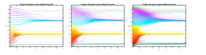
    Evolution of the positions for N=20, N=50 and N=100. The thickness of the lines is proportional to the agent's weight. The dotted line represents the barycenter ˉx:=1Mimixi

    .
    Figure 2. 

    Evolution of the weights for N=20, N=50 and N=100. The dotted line represents the average weight ˉm:=1Mimi

    .
    Figure 3. 

    Comparison of μt (in red), solution to the macroscopic model (33) and ˜μNt (in blue), counting measure corresponding to the solution to the microscopic model (32) for N=100

    .

    ϕ:=ϕ0.2, where for all R>0, ϕR:δδ|δ|sin2(πR|δ|)1|δ|R,

    h:δarctan(|δ|)δ|δ|,

    dμ0(x):=f(x)Fdx, with

    f(x):=[3.50.4πexp(5(x0.25)24)+10.4πexp(5(x0.90)24)]1[0,1](x)

    and F:=Rf(x)dx.

    Remark 5. The interaction function ϕR provides an example of a bounded- confidence model (see [15]): agents interact only if they are within distance R of one another. Furthermore, the force exerted by xj on xi is colinear to the vector xjxi: this translates the fact that xj attracts xi. Since the seminal paper [15], bounded-confidence models have been extensively studied in opinion dynamics, and it is well-known that they can lead to various global phenomena such as consensus or clustering.

    Figure 1 shows the evolution of t(xNi(t))i{1,,N} and Figure 2 shoes the evolution of t(mNi(t))i{1,,N} for N=20, N=50 and N=100. Due to the fact that the interaction function ϕ has compact support, we observe formation of clusters within the population. Note that as expected, the final number and positions of clusters are the same for all values of N (N big enough). Within each cluster, the agents that are able to attract more agents gain influence (i.e. weight), while the followers tend to lose influence (weight).

    Figure 3 compares the evolutions of tμt and tμNt at four different times. For visualization, the empirical measure was represented by the piece-wise constant counting measure ˜μNt defined by: for all xEj, ˜μNt(x)=pMNi=1mi1{xiEj}, where for each j{1,,p}, Ej=[j1p,jp), so that (Ej)j{1,,p} is a partition of [0,1]. In Fig. 3, p=41. We observe a good correspondence between the two solutions at all four time steps. Observe that the four clusters are formed at the same locations that in Figure 1, i.e. at x=0.07, x=0.33, x=0.66 and x=0.9. Convergence to the first and fourth clusters is slower than convergence to the second and third, due to the differences in the total weight of each cluster.

    We provide the proof of Proposition 2. It is modeled after the proof of existence and uniqueness of the Graph Limit equation provided in [2], but we write it fully here for self-containedness.

    Proof. Let (˜xi)i{1,,N}C([0,T];(Rd)N) and (˜mi)i{1,,N}C([0,T];RN+). Consider the following decoupled systems of ODE:

    {˙xi(t)=1MNj=1˜mj(t)ϕ(xj(t)xi(t)),xi(0)=xini; (34)
    {˙mi(t)=mi(t)1MqNj1=1Njq=1mj1(t)mjq(t)S(˜xi(t),˜xj1(t),˜xjq(t)),mi(0)=mini. (35)

    Existence and uniqueness of the solution to the Cauchy problem given by (34) comes from a simple fixed-point argument.

    We now show existence and uniqueness of the solution to the second decoupled system (35). Let m0RN+ such that Ni=1mini=M. Let Mmin:={mC([0,˜T],RN+)|m(t=0)=min and Ni=1miM}. Consider the application Kmin:MminMmin where

    (Kminm)i(t):=m0i+t0mi(τ)1MqNj1=1Njq=1mj1(τ)mjq(τ)S(˜xi(τ),˜xj1(τ),˜xjq(τ))dτ

    for all t[0,˜T] and i{1,,N}. We show that Kmin is contracting for the norm mMmin:=1Msupt[0,˜T]Ni=1|mi(t)|. Let m,pMmin. It holds:

    |(KminmKminp)i|t01Mq|mipi|j1jqmj1mjq|S(˜xi,˜xj1,˜xjq)|dτ+t01Mqpij1jq|mj1pj1|mj2mjq|S(˜xi,˜xj1,˜xjq)|dτ++t01Mqpij1jqpj1pjq1|mjqpjq||S(˜xi,˜xj1,˜xjq)|dτˉS˜Tsup[0,˜T]|mipi|+qˉS˜T1Msup[0,˜T](piNj=1|mjpj|)ˉS˜Tsup[0,˜T]|mipi|+qˉS˜Tsup[0,˜T]Nj=1|mjpj|.

    Thus, KminmKminpMmin(q+1)ˉS˜TmpMmin. Taking ˜T12((q1)ˉS)1, the operator Kmin is contracting. Thus, there is a unique solution mC1([0,T],RN+) to (35).

    Let us define the sequences (xn)nN and (mn)nN by : m0(t)=min and x0(t)=xin for all t[0,T]. For all n1, xn and mn are solutions to the system of ODEs

    ˙xni=1MNj=1mn1jϕ(xnjxni),˙mni=mni1MqNj1=1Njq=1mnj1mnjqS(xn1i,xn1j1,xn1jq)

    with initial conditions xni(0)=xini and mni(0)=mini. The results obtained above ensure that the sequences are well defined and that for all nN, (xn,mn)C([0,T];(Rd)N×RN+). We begin by showing that xn and mn are bounded in L norm independently of n. It holds: |mni(t)||mini|+ˉSt0|mni(τ)|dτ. From Gronwall's lemma, for all t[0,T], |mni(t)|minieˉStMT where MT:=maxi{1,,N}minieˉST.

    Similarly, notice that for all zRd, ϕ(z)Φ0+Lϕz, where Φ0=ϕ(0). Then xni(t)xini+MTMt0Nj=1(Φ0+2Lϕmaxi{1,,N}xni(τ))dτ. Thus

    maxi{1,,N}xni(t)maxi{1,,N}xini+MTM(Φ0t+2Lϕt0maxi{1,,N}xni(τ)dτ)

    and from Gronwall's lemma, for all t[0,T],

    maxi{1,,N}xni(t)XT:=[maxi{1,,N}xini+MTMΦ0T]e2LϕMTMT.

    We prove that (xn)nN and (mn)nN are Cauchy sequences. For all nN,

    xn+1ixni=t01MNj=1mnjϕ(xn+1jxn+1i)dτt01MNj=1mn1jϕ(xnjxni)dτ
    1M(Φ0+2LϕXT)t0Nj=1|mnjmn1j|dτ+MTLϕMt0Nj=1(xn+1jxnj+xn+1ixni)dτ.

    Thus

    ixn+1ixniNM(Φ0+2LϕXT)t0i|mnimn1i|dτ+2NMTLϕMt0ixn+1ixnidτ.

    A similar computation, for m gives

    |mn+1imni|t0|mn+1imni|1Mqj1jqmn+1j1mn+1jqS(xnixnjq)dτ+t0mni1Mqj1jq|mn+1j1mnj1|mn+1j2mn+1jqS(xnixnjq)dτ++t0mni1Mqj1jqmnj1mnjq1|mn+1jqmnjq|S(xnixnjq)dτ+t0mni1Mqj1jqmnj1mnjq|S(xnixnjq)S(xn1ixn1jq)|dτ.

    From (9), it holds t0mni1Mqj1jqmnj1mnjq|S(xnixnjq)S(xn1ixn1jq)|dτt0mniLSxnixn1idτ+qt01MNj=1mnjLSxnjxn1jdτ.

    Thus, |mn+1imni|ˉSt0|mn+1imni|dτ+qˉSMTMt0j|mn+1jmnj|dτ+MTt0LSxnixn1idτ+qLSMTMt0jxnjxn1jdτ. Summing the terms, it holds

    Ni=1|mn+1imni|ˉS(1+qNMTM)t0Nj=1|mn+1jmnj|dτ+MTLS(1+qNM)t0Ni=1xnjxn1jdτ.

    Summarizing, we have

    Ni=1xn+1ixniC1t0Ni=1xn+1ixnidτ+C2t0Ni=1|mnimn1i|dτ;Ni=1|mn+1imni|C3t0Ni=1|mn+1imni|dτ+C3t0Ni=1xnixn1idτ.

    where C1=2NMTLϕM, C2=NM(Φ0+2LϕXT), C3=ˉS(1+qNMTM) and C4=MTLS(1+qNM). Let un:=Ni=1xn+1ixni+Ni=1|mn+1imni| for all nN. Then un(t)ATt0un(τ)dτ+ATt0un1(τ)dτ where AT:=max(C1,C2,C3,C4). From Gronwall's lemma, for all t[0,T], un(t)ATeATTt0un1(τ)dτ which, by recursion, implies un(t)(ATeATT)nn!sup[0,T]u0. This is the general term of a convergent series. Thus, for all n,pN,

    Ni=1xn+pixnin+p1k=nNi=1xk+1ixkin+p1k=nukn,p+0.

    This proves that (xn)nN is a Cauchy sequence in the Banach space C([0,T],(Rd)N) for the norm xsupt[0,T]Ni=1xni(t). Similarly, (mn)nN is a Cauchy sequence in C([0,T],RN+) for the norm msupt[0,T]Ni=1|mni(t)|. One can easily show that their limits (x,m) satisfy the system of ODEs (3). Furthermore, since the bounds XT and MT do not depend on n, it holds xi(t)XT and |mi(t)|MT for all t[0,T] and every i{1,,N}. This concludes the proof of existence.

    Let us now deal with uniqueness. Suppose that (x,m) and (p,m) are two couples of solutions to the Cauchy problem (3) with the same initial conditions (xin,min). As previously,

    Ni=1xi(t)yi(t)+Ni=1|mi(t)pi(t)|ATt0(Ni=1xi(τ)yi(τ)+Ni=1|mi(τ)pi(τ)|)dτ.

    By Gronwall's lemma, Ni=1xi(t)yi(t)+Ni=1|mi(t)pi(t)|=0, which concludes uniqueness.


    [1] A simulation study on the schooling mechanism in fish. Nippon Suisan Gakkaishi (1982) 48: 1081-1088.
    [2] Mean-field and graph limits for collective dynamics models with time-varying weights. Journal of Differential Equations (2021) 299: 65-110.
    [3]

    W. Braun and K. Hepp, The Vlasov dynamics and its fluctuations in the 1/N limit of interacting classical particles, Communications in Mathematical Physics, 56 (1977), 101–113, URL https://projecteuclid.org:443/euclid.cmp/1103901139.

    [4]

    F. Bullo, J. Cortés and S. Martínez, Distributed Control of Robotic Networks: A Mathematical Approach to Motion Coordination Algorithms, Princeton Series in Applied Mathematics. Princeton University Press, Princeton.

    [5] A Eulerian approach to the analysis of rendez-vous algorithms. IFAC Proceedings Volumes (2008) 41: 9039-9044.
    [6] Emergent behavior in flocks. IEEE Transactions on Automatic Control (2007) 52: 852-862.
    [7]

    P. Degond, Macroscopic limits of the Boltzmann equation: A review, Birkhäuser Boston, Boston, MA, 2004, 3–57.

    [8] Large scale dynamics of the persistent turning walker model of fish behavior. Journal of Statistical Physics (2008) 131: 989-1021.
    [9] Reaching a consensus. Journal of American Statistical Association (1974) 69: 118-121.
    [10] Vlasov equations. Functional Analysis and Its Applications (1979) 13: 115-123.
    [11]

    R. M. Dudley, Real Analysis and Probability, 2nd edition, Cambridge Studies in Advanced Mathematics, Cambridge University Press, 2002.

    [12] A formal theory of social power. Psychological Review (1956) 63: 181-194.
    [13] Collective behavior in animal groups: Theoretical models and empirical studies. Human Frontier Science Program Journal (2008) 2: 205-219.
    [14] From particle to kinetic and hydrodynamic descriptions of flocking. Kinetic and Related Models (2008) 1: 415-435.
    [15]

    R. Hegselmann, U. Krause et al., Opinion dynamics and bounded confidence models, analysis, and simulation, Journal of Artificial Societies and Social Simulation, 5.

    [16] Social dynamics models with time-varying influence. Mathematical Models and Methods in Applied Sciences (2019) 29: 681-716.
    [17]

    B. Piccoli and N. Pouradier Duteil, Control of collective dynamics with time-varying weights, in Recent Advances in Kinetic Equations and Applications (ed. F. Salvarani), Springer International Publishing, Cham, 2021,289–308.

    [18] Generalized Wasserstein distance and its application to transport equations with source. Archive for Rational Mechanics and Analysis (2014) 211: 335-358.
    [19] On properties of the generalized wasserstein distance. Archive for Rational Mechanics and Analysis (2016) 222: 1339-1365.
    [20]

    B. Piccoli and F. Rossi, Measure-theoretic models for crowd dynamics, Springer International Publishing, Cham, 2018,137–165.

    [21]

    B. Piccoli, F. Rossi and M. Tournus, A Wasserstein norm for signed measures, with application to nonlocal transport equation with source term, HAL, (2019), URL https://hal.archives-ouvertes.fr/hal-01665244, arXiv: 1910.05105.

    [22] Novel type of phase transition in a system of self-driven particles. Physical Review Letters (1995) 75: 1226-1229.
    [23]

    C. Villani, Optimal Transport: Old and New, Grundlehren der mathematischen Wissenschaften, Springer Berlin Heidelberg, 2008.

  • This article has been cited by:

    1. Benedetto Piccoli, Nastassia Pouradier Duteil, 2021, Chapter 12, 978-3-030-82945-2, 289, 10.1007/978-3-030-82946-9_12
    2. Yurii Averboukh, Nonlocal Balance Equation: Representation and Approximation of Solution, 2024, 1040-7294, 10.1007/s10884-024-10373-8
    3. Rico Berner, Thilo Gross, Christian Kuehn, Jürgen Kurths, Serhiy Yanchuk, Adaptive dynamical networks, 2023, 1031, 03701573, 1, 10.1016/j.physrep.2023.08.001
    4. Marvin Lücke, Jobst Heitzig, Péter Koltai, Nora Molkenthin, Stefanie Winkelmann, Large population limits of Markov processes on random networks, 2023, 166, 03044149, 104220, 10.1016/j.spa.2023.09.007
    5. Immanuel Ben-Porat, José A. Carrillo, Pierre-Emmanuel Jabin, The graph limit for a pairwise competition model, 2024, 413, 00220396, 329, 10.1016/j.jde.2024.08.069
    6. Martin Gugat, Michael Herty, Chiara Segala, The turnpike property for mean-field optimal control problems, 2024, 35, 0956-7925, 733, 10.1017/S0956792524000044
    7. Immanuel Ben-Porat, José A. Carrillo, Sondre T. Galtung, Mean field limit for one dimensional opinion dynamics with Coulomb interaction and time dependent weights, 2024, 240, 0362546X, 113462, 10.1016/j.na.2023.113462
    8. Nathalie Ayi, Nastassia Pouradier Duteil, 2024, Chapter 3, 978-3-031-73422-9, 79, 10.1007/978-3-031-73423-6_3
    9. Antonio Esposito, Georg Heinze, André Schlichting, Graph-to-local limit for the nonlocal interaction equation, 2025, 00217824, 103663, 10.1016/j.matpur.2025.103663
    10. N. I. Pogodaev, M. V. Staritsyn, Optimal Control of Nonlocal Balance Equations in the Space of Nonnegative Measures, 2025, 66, 0037-4466, 576, 10.1134/S0037446625020223
  • Reader Comments
  • © 2022 the Author(s), licensee AIMS Press. This is an open access article distributed under the terms of the Creative Commons Attribution License (http://creativecommons.org/licenses/by/4.0)
通讯作者: 陈斌, bchen63@163.com
  • 1. 

    沈阳化工大学材料科学与工程学院 沈阳 110142

  1. 本站搜索
  2. 百度学术搜索
  3. 万方数据库搜索
  4. CNKI搜索

Metrics

Article views(1409) PDF downloads(190) Cited by(10)

Other Articles By Authors

/

DownLoad:  Full-Size Img  PowerPoint
Return
Return

Catalog