An inverse problem for quantum trees with observations at interior vertices

Sergei Avdonin; Julian Edward; Sergei Avdonin; Julian Edward

doi:10.3934/nhm.2021008

Networks and Heterogeneous Media

2021, Volume 16, Issue 2: 317-339. doi: 10.3934/nhm.2021008

Previous Article Next Article

An inverse problem for quantum trees with observations at interior vertices

Sergei Avdonin ^{1
,},
Julian Edward ^{2
,
,}

1.
Department of Mathematics and Statistics, University of Alaska at Fairbanks, Fairbanks, AK 99775, USA
2.
Department of Mathematics and Statistics, Florida International University, Miami, FL 33199, USA

Received: 01 April 2020 Revised: 01 January 2021 Published: 12 March 2021
Primary: 35R30; Secondary: 35R02, 35L05, 35L20

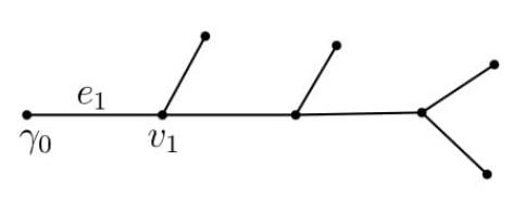
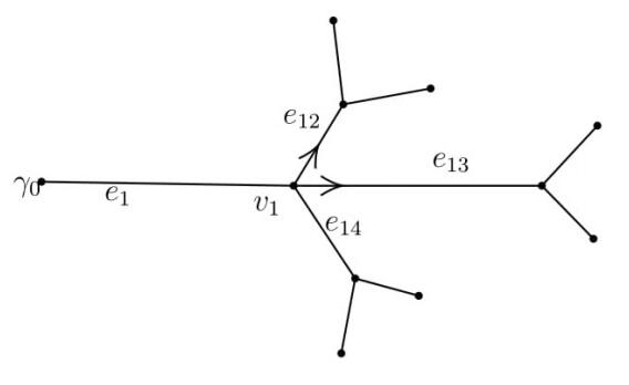
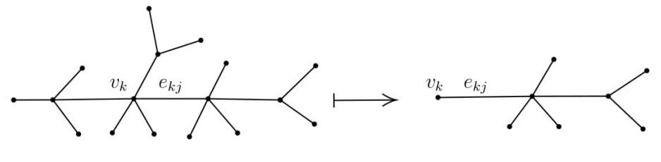
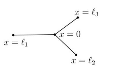
In this paper we consider a non-standard dynamical inverse problem for the wave equation on a metric tree graph. We assume that positive masses may be attached to the internal vertices of the graph. Another specific feature of our investigation is that we use only one boundary actuator and one boundary sensor, all other observations being internal. Using the Dirichlet-to-Neumann map (acting from one boundary vertex to one boundary and all internal vertices) we recover the topology and geometry of the graph, the coefficients of the equations and the masses at the vertices.
- Inverse problem,
- quantum graph,
- wave equation,
- boundary and interior measurements,
- attached masses
Citation: Sergei Avdonin, Julian Edward. An inverse problem for quantum trees with observations at interior vertices[J]. Networks and Heterogeneous Media, 2021, 16(2): 317-339. doi: 10.3934/nhm.2021008

Related Papers:

Abstract

In this paper we consider a non-standard dynamical inverse problem for the wave equation on a metric tree graph. We assume that positive masses may be attached to the internal vertices of the graph. Another specific feature of our investigation is that we use only one boundary actuator and one boundary sensor, all other observations being internal. Using the Dirichlet-to-Neumann map (acting from one boundary vertex to one boundary and all internal vertices) we recover the topology and geometry of the graph, the coefficients of the equations and the masses at the vertices.

References

[1]	A self-consistent theory for graphene transports. Proc. Natl. Acad. Sci. USA (2007) 104: 18392-18397.
[2]	Control and inverse problems for networks of vibrating strings with attached masses. Nanosystems: Physics, Chemistry, and Mathematics (2016) 7: 835-841.
[3]	Parabolic differential-algebraic models in electrical network design. Multiscale Model. Simul. (2005) 4: 813-838.
[4]	Control, observation and identification problems for the wave equation on metric graphs. IFAC-PapersOnLine (2019) 52: 52-57.
[5]	S. Avdonin, Using hyperbolic systems of balance laws for modeling, control and stability analysis of physical networks, in Analysis on Graphs and Its Applications (Proceedings of Symposia in Pure Mathematics), 77, AMS, Providence, RI, 2008,507–521.
[6]	S. Avdonin, N. Avdonina and J. Edward, Boundary inverse problems for networks of vibrating strings with attached masses, in Dynamic Systems and Applications, 7, Dynamic, Atlanta, GA, 2016, 41–44.
[7]	Determining a distributed conductance parameter for a neuronal cable model defined on a tree graph. Inverse Probl. Imaging (2015) 9: 645-659.
[8]	An inverse problem for quantum trees with delta-prime vertex conditions. Vibration (2020) 3: 448-463.
[9]	Controllability for a string with attached masses and Riesz bases for asymmetric spaces. Math. Control Relat. Fields (2019) 9: 453-494.
[10]	Exact controllability for string with attached masses. SIAM J. Control Optim. (2018) 56: 945-980.
[11]	Inverse problems for quantum trees. Inverse Probl. Imaging (2008) 2: 1-21.
[12]	Inverse problems for quantum trees II: Recovering matching conditions for star graphs. Inverse Probl. Imaging (2010) 4: 579-598.
[13]	On an inverse problem for tree-like networks of elastic strings. ZAMM Z. Angew. Math. Mech. (2010) 90: 136-150.
[14]	S. Avdonin and V. Mikhaylov, The boundary control approach to inverse spectral theory, Inverse Problems, 26 (2010), 19pp. doi: 10.1088/0266-5611/26/4/045009
[15]	S. Avdonin and S. Nicaise, Source identification problems for the wave equation on graphs, Inverse Problems, 31 (2015), 29pp. doi: 10.1088/0266-5611/31/9/095007
[16]	S. Avdonin and Y. Zhao, Exact controllability of the 1-D wave equation on finite metric tree graphs, Appl. Math. Optim., (2019). doi: 10.1007/s00245-019-09629-3
[17]	Leaf peeling method for the wave equation on metric tree graphs. Inverse Probl. Imaging (2021) 15: 185-199.
[18]	Boundary control and an inverse matrix problem for the equation $u_tt-u_xx+V(x)u = 0$. Math. USSR-Sb. (1992) 72: 287-310.
[19]	(1995) Families of Exponentials. The Method of Moments in Controllability Problems for Distributed Parameter Systems. Cambridge: Cambridge University Press.
[20]	On inverse dynamical and spectral problems for the wave and Schrödinger equations on finite trees. The leaf peeling method. J. Math. Sci. (NY) (2017) 224: 1-10.
[21]	G. Bastin, J. M. Coron and B. d'Andrèa Novel, Using hyperbolic systems of balance laws for modeling, control and stability analysis of physical networks, in Proceedings of the Lecture Notes for the Pre-Congress Workshop on Complex Embedded and Networked Control Systems, 17th IFAC World Congress, Seoul, Korea, 2008, 16–20.
[22]	Boundary spectral inverse problem on a class of graphs (trees) by the BC method. Inverse Problems (2004) 20: 647-672.
[23]	Inverse problems on graphs: Recovering the tree of strings by the BC-method. J. Inverse Ill-Posed Probl. (2006) 14: 29-46.
[24]	A distributed parameter identification problem in neuronal cable theory models. Math. Biosci. (2005) 194: 1-19.
[25]	G. Berkolaiko and P. Kuchment, Introduction to Quantum Graphs, Mathematical Surveys and Monographs, 186, American Mathematical Society, Providence, RI, 2013. doi: 10.1090/surv/186
[26]	Analysis of a graph by a set of automata. Program. Comput. Softw. (2015) 41: 307-310.
[27]	Parallel computations on a graph. Program. Comput. Softw. (2015) 41: 1-13.
[28]	A Borg-Levinson theorem for trees. Proc. R. Soc. Lond. Ser. A Math. Phys. Eng. Sci. (2005) 461: 3231-3243.
[29]	Optimal control in networks of pipes and canals. SIAM J. Control Optim. (2009) 48: 2032-2050.
[30]	R. Dáger and E. Zuazua, Wave Propagation, Observation and Control in 1-$d$ Flexible Multi-Structures, Mathematics & Applications, 50, Springer-Verlag, Berlin, 2006. doi: 10.1007/3-540-37726-3
[31]	P. Exner, Vertex couplings in quantum graphs: Approximations by scaled Schrödinger operators, in Mathematics in Science and Technology, World Sci. Publ., Hackensack, NJ, 2011, 71–92. doi: 10.1142/9789814338820_0004
[32]	Inverse problems for differential operators on trees with general matching conditions. Appl. Anal. (2007) 86: 653-667.
[33]	Global boundary controllability of the Saint-Venant system for sloped canals with friction. Ann. Inst. H. Poincaré Anal. Non Linéaire (2009) 26: 257-270.
[34]	Can you hear the shape of a graph?. J. Phys. A. (2001) 34: 6061-6068.
[35]	Output feedback stabilization of a tree-shaped network of vibrating strings with non-collocated observation. Internat. J. Control (2011) 84: 458-475.
[36]	Exact controllability and stabilization of a vibrating string with an interior point mass. SIAM J. Control Optim. (1995) 33: 1357-1391.
[37]	N. E. Hurt, Mathematical Physics of Quantum Wires and Devices, Mathematics and its Applications, 506, Kluwer Academic Publishers, Dordrecht, 2000. doi: 10.1007/978-94-015-9626-8
[38]	C. Joachim and S. Roth, Atomic and Molecular Wires, NATO Science Series E, 341, Springer Netherlands, 1997.
[39]	Kirchoff's rule for quantum wires. J. Phys. A (1999) 32: 595-630.
[40]	Kirchoff's rule for quantum wires. II. The inverse problem with possible applications to quantum computers. Fortschr. Phys. (2000) 48: 703-716.
[41]	Periodic orbit theory and spectral statistics for quantum graphs. Ann. Physics (1999) 274: 76-124.
[42]	Quantum chaos on graphs. Phys. Rev. Lett. (1997) 79: 4794-4797.
[43]	Inverse spectral problem for quantum graphs. J. Phys. A. (2005) 38: 4901-4915.
[44]	J. E. Lagnese, G. Leugering and E. J. P. G. Schmidt, Modeling, Analysis and Control of Dynamical Elastic Multi-Link Structures, Systems & Control: Foundations & Applications, Birkhäuser Boston, Inc., Boston, MA, 1994. doi: 10.1007/978-1-4612-0273-8
[45]	Two-body scattering on a graph and application to simple nanoelectronic devices. J. Math. Phys. (1995) 36: 2813-2825.
[46]	N. M. R. Peres, Scattering in one-dimensional heterostructures described by the Dirac equation, J. Phys. Condens. Matter, 21 (2009). doi: 10.1088/0953-8984/21/9/095501
[47]	N. M. R. Peres, J. N. B. Rodrigues, T. Stauber and J. M. B. Lopes dos Santos, Dirac electrons in graphene-based quantum wires and quantum dots, J. Phys. Condens. Matter, 21 (2009). doi: 10.1088/0953-8984/21/34/344202
[48]	W. Rall, Core conductor theory and cable properties of neurons, in Handbook of Physiology, The Nervous System, Cellular Biology of Neurons, American Physiological Society, Rockville, MD, 1977, 39–97. doi: 10.1002/cphy.cp010103
[49]	Inverse spectral problems for Sturm-Liouville operators on graphs. Inverse Problems (2005) 21: 1075-1086.
[50]	E. Zuazua, Control and stabilization of waves on 1-d networks, in Modelling and Optimisation of Flows on Networks, Lecture Notes in Math., 2062, Springer, Heidelberg, 2013,463–493. doi: 10.1007/978-3-642-32160-3_9

Reader Comments

Your name:*

Email:*
© 2021 the Author(s), licensee AIMS Press. This is an open access article distributed under the terms of the Creative Commons Attribution License (http://creativecommons.org/licenses/by/4.0)