1.
Introduction
In this paper we are investigating finite and infinite systems of strings or beams having a common endpoint, whose transversal vibrations may take place in different planes. We are interested in conditions ensuring their simultaneous observability and in estimating the sufficient observability time.
There have been many results during the last twenty years on the simultaneous observability and controllability of systems of strings and beams, see e.g., [1]-[6], [11]-[12], [20], [25]. In all earlier papers the vibrations were assumed to take place in a common vertical plane. Here, we still assume that each string or beam is vibrating in some plane, but these planes may differ from one another. This leads to important new difficulties, requiring vectorial generalizations of clasical Ingham type theorems. Our approach also allows us to consider infinite systems of strings or beams, which requires a deeper study of the overall density of the union of all corresponding eigenfrequencies.
For a general introduction to the controllability of PDE's we refer to [22,23] or [18]. The approach of the present paper is based on some classical results of Ingham [14], Beurling [9] and Kahane [17] on nonharmonic analysis. Some of the first applications to control thery were given in the papers of Ball and Slemrod [7] and Haraux [13]. We refer to [19] for a general introduction.
The paper is organized as follows. Section 2 is devoted to the statement of our main results. In Section 3 we briefly recall out harmonic analysis tools on which the proofs of our main theorems are based. The remaining part of the paper is devoted to the proofs of the results. In particular, the theorems concerning the observability of string systems (Theorems 2.1, 2.2 and 2.3) are proved in Sections 4 and 5. In Section 6 we prove Theorem 2.4 on the observability of infinite beam systems under some algebraic conditions on the lengths of the beams. Finally in Section 7 we prove Proposition 1 providing many examples where the hypotheses of Theorem 2.4 are satisfied.
2.
Main results
In what follows we state our main results on the simultaneous observability of string and beam systems.
2.1. Simultaneous observability of string systems.
We consider a system of J<∞ vibrating strings of length ℓj, 1≤j≤J. The problem is set in the spherical coordinate system (r,φ,θ)∈[0,∞)×R×(−π2,π2]. The direction of the j-th string is dj:=(ℓj,φj,θj): this, together with an unit vector vj in R3 orthogonal to dj, is fixed by initial data. The transversal displacement of the j-th string at time t and at the point (r,φj,θj) for r∈[0,ℓj] is denoted by uj(t,r,φj,θj)vj.
We consider the following uncoupled system:
(As usual, the subscripts t and r denote differentiations with respect to these variables.) It is well-known that the system is well posed for
and the corresponding functions t↦uj,r(t,0,φj,θj) are locally square integrable ("hidden regularity").
We seek conditions ensuring that the linear map
of the Hilbert space H:=∏Jj=1H10(0,ℓj)×L2(0,ℓj) into L2loc(R;R3) is one-to-one. If this is so, then we would also like to obtain more precise, quantitative norm estimates.
Setting
for brevity, the solutions of (1) are given by the formulas
with suitable complex coefficients bj,±k, and
The linear map (2) is not always one-to-one. Indeed, if there exists a real number ω such that the set of vectors
is linearly dependent, then denoting by J′ the set of the corresponding indices j and choosing a nontrivial (finite) linear combination
the functions
define a non-trivial solution of (1) satisfying
so that the linear map (2) on H is not one-to-one.
A positive observability result is the following:
Theorem 2.1. Assume that
Then there exists a number
such that the restricted linear map
where u1,…,uJ are solutions of (1), is one-to-one for every interval I of length >T0, and for no interval I of length <T0.
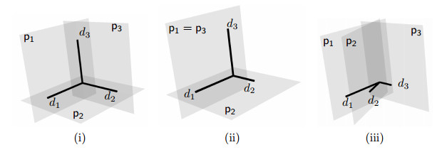
Remark 1. The proof of Theorem 2.1 yields a more precise estimation of T0 in some special cases (see Remark 7 below). We give three examples.
(ⅰ) If J=3 and v1,v2,v3 are mutually orthogonal, then T0=2max{ℓ1,ℓ2,ℓ3}, see Figure 1-(i).
(ⅱ) If J=3 and v1⊥v2=v3, then T0=2max{ℓ1+ℓ2,ℓ3}, see Figure 1-(ii).
(ⅲ) If all vectors vj are equal (we call this the planar case), then T0=2(ℓ1+⋯+ℓJ)– see Figure 1-(iii). Thus we recover an earlier theorem in [5,6] by using Fourier series. It was also proved in [11] by a method based on d'Alembert's formula. The method of Fourier series enables us to consider more general equations of the type uj,tt−uj,rr+ajuj=0 in (1) with arbitrary nonnegative constants (d'Alembert's formulas cannot be generalized to the case where aj≠0). Moreover, we may even consider infinitely many strings.
Incidentally note that if the vectors vj are linearly independent then we do not need the assumption (3). But this may only happen if we have at most three vectors, while the interest of the present paper is to have many, maybe even infinitely many strings or beams, and thus many vectors vj.
Under some further assumptions on the lengths of the strings we may also get explicit norm estimates. We adopt the following notations. For each fixed j≥1, let
be the usual orthonormal basis of L2(0,ℓj). We denote by Ds(0,ℓj) the Hilbert spaces obtained by completion of the linear hull of (ej,k) with respect to the Euclidean norm
Note that, identifying L2(0,ℓj) with its dual, we have
with equivalent norms.
Theorem 2.2. Consider the system (1). Assume that all ratios ℓj/ℓm with j≠m are quadratic irrational numbers. Then there exists a constant c>0 such that the solutions of (4) satisfy estimates
for every bounded interval I of length |I|>2∑Jj=1ℓj.
Next we consider a more general system with given real numbers aj≥0, and ℓj>0:
For any given initial data
the system has a unique solution, given by the formula
where now we use the notation
Theorem 2.3. Assume that
Then the restricted linear map
where u1,…,uJ are solutions of (4), is well defined and continuous from H into L2(I;R3) for every bounded interval I.
Moreover, there exists a number
such that the map (7) is one-to-one for every interval I of length >T0, and for no interval of length <T0.
Remark 2.
(ⅰ) If aj=0 for all j, then the condition (6) is equivalent to (3).
(ⅱ) We may wonder whether Theorems 2.1, 2.2 and 2.3 remain valid for infinite string systems having a finite total length if the observability time is greater than 2∑∞j=1ℓj. we will show in Remark 8 below that our proofs cannot be adapted to prove such results.
2.2. Simultaneous observability of beam systems
Our approach may be adapted to systems of hinged beams. Moreover, we may even consider systems of infinitely many beams. We consider the following system:
For any given initial data
the system has a unique solution, given by the formula
where now we use the notation
Let us denote by H the vector space of those sequences (9) that satisfy the condition
The formula
defines a Euclidean norm on H for which H becomes a Hilbert space.
Henceforth we consider the solutions of (8) for initial data belonging to H.
Theorem 2.4. Assume that
Furthermore, assume that there exists a constant A>0 such that
whenever j≠m.
Then there exist a number T0≥0 and a constant c>0 such that the solutions of (8) satisfy the relation
for every bounded interval I of length >T0, where uj with j=1,2,… are the solutions of (8).
It is not obvious that there exist infinite sequences (ℓj) satisfying (10) and (11). We give three different examples.
We recall that a Perron number is a real algebraic integer q of degree ≥2 whose conjugates are all smaller than q in absolute value. For example, the Golden Ratio q≈1.618 and more generally the Pisot and Salem numbers are Perron numbers. In what follows we use the symbol [x] to denote the lower integer part of x.
Proposition 1. The sequence (ℓj)∞j=1 satisfies (10) and (11) in the following three cases:
(ⅰ) q is a quadratic Perron number and ℓj=q−j;
(ⅱ) ℓj=12j+√2;
(ⅲ) ℓj=πj+1+√2.
Remark 3.
(ⅰ) The conclusion of Theorem 2.4 remains valid for systems of Schrödinger equations of the form
(we may also change some uj,t+iuj,rr=0 to uj,t−iuj,rr=0 for some or all indices j) because every solution of (12) also satisfies (8): see, e.g., [18,Section 6.4,p. 82].
(ⅱ) The beams in Proposition 1 (iii) have an infinite total length. Since we have an infinite propagation speed for beams (see [18,Theorem 6.7]), this does not exclude the observability of the system.
(ⅲ) We conjecture that T0=0 in all cases covered by Proposition 1.
3.
Review of some Ingham type theorems
We recall some tools we need in this paper. We refer to [19] for more details and proofs. Every increasing sequence (ωk)k∈Z of real numbers has an upper density
where n+(r) denotes the largest number of terms of the sequence (ωk)k∈Z contained in an interval of length r. It is shown in [6,Proposition 1.4] that the upper density is finite if and only if the following weakened gap condition is satisfied: there exists an integer M≥1 and a real number γ>0 such that
(This proposition is crucial for enabling us to consider infinite string and beam systems.)
If the sequence is uniformly separated, i.e., if (13) is satisfied with M=1 (uniform gap condition), then D+≤1γ.
First we state a vectorial generalization of Parseval's formula. Given two expressions A(u) and B(u) depending on the solutions henceforth we write A≲ or if with some constant , independent of the choice of the particular solution. Furthermore, we write if and .
Theorem 3.1. Let be a uniformly separated increasing sequence with upper density , a sequence of unit vectors in some complex Hilbert space , and a bounded interval of length .
(ⅰ) The functions
are well defined in for all square summable sequences of complex numbers, and
(ⅱ) If , then the inverse inequality also holds:
Proof. The scalar case is classical, due to Ingham [14] and Beurling [9]; see also [17] for higher-dimensional generalizations. In the general case we choose an orthonormal basis of the linear hull of in , and we write with suitable complex numbers . Then we have
Applying the scalar case of the theorem to each integral on rifght hand side, and using the Bessel equality
for every , the theorem follows.
Remark 4. In the scalar case Beurling proved that the value is the best possible. In the vectorial case the best possible value may be smaller: see [8].
Next we recall from [6] (see also [19,Theorem 9.4]) a generalization of the scalar case of Theorem 3.1 for arbitrary increasing sequences having a finite upper density:
Theorem 3.2. Let be an increasing sequence with a finite upper density , and a bounded interval of length .
(ⅰ) The functions
are well defined in for all square summable sequences of complex numbers, and
(ⅱ) There exists another basis of the linear span of the functions such that if we rewrite the functions in this basis:
then
and
whenever .
Remark 5. The value is still the best possible: see [25].
Remark 6. In fact, the theorem in [6] is more precise because the new basis is explicitly defined by Newton's formula of divided differences. Hence there is an estimate between the coefficients and . To explain this, let be an increasing sequence satisfying the weakened gap condition (13), and fix arbitrarily. Then we may partition the sequence into disjoint finite subsequences with , such that
but
For each such group we define the divided differences of the exponential functions by the formula
Then we have
with an invertible linear transformation
Furthermore, we may infer from the structure of the divided differences that whenever , and there exists a constant such that
for all with .
We end this section by stating a consequence of Theorem 3.2 for vector valued functions.
Corollary 1. Let be an increasing sequence with a finite upper density , a sequence of unit vectors in some complex Hilbert space , and a bounded interval of length .
(ⅰ) The functions
are well defined in for all square summable sequences of complex numbers, and
(ⅱ) If for all for some interval of length , then all coefficients vanish.
Proof. Choosing an orthonormal basis of the linear hull of , and writing with suitable complex numbers as in the proof of Theorem 3.1, we have
and
for every .
(i) Applying Theorem 3.2 (i) to each integral on the right hand side of (14), and using (15), we have
We have used here the fact that the hidden constants in the relations do not depend on because we apply Theorem 3.2 for the same exponent sequence .
(ii) Applying Theorem 3.2 (ii) to each integral on the right hand side of (14) we obtain that for all and . Since for all , for each there exists such that , and therefore .
Remark 7. Let us introduce the sets
The proof of Corollary 1 (see (14)) shows that we may replace by
4.
Proof of Theorems 2.1 and 2.3
We only prove Theorem 2.3 because Theorem 2.1 is similar and simpler. It follows by an elementary consideration using translation invariance that there exists a value such that the uniqueness property in Theorem 2.3 holds on every interval of length , and it fails on every interval of length .
We recall that the solution of (4) have the form
with
Hence
Furthermore, we obtain by a direct computation that
and
whence
(We have an equality if for all .) Thanks to assumption (6) we may combine all exponents into a unique increasing sequence . Setting if , the theorem will follow from (16) and (17) with some by applying Corollary 1 and the following
Lemma 4.1. The sequence has a finite upper density .
Proof. Since as , each set
has the upper density . Moreover, every interval of length contains
elements of . Therefore
It remains to show that for every . For any fixed , given an arbitrary interval of length , by a well-known classical result (see for instance [18,Ch. 3]) on the one-dimensional wave equation there exists a non-trivial solution of the problem
such that
Choosing to be identically zero for all , we obtain a non-trivial solution of the system (4) for which the right hand side of (7) vanishes on .
5.
Proof of Theorem 2.2
Instead of (17) now we have for every real number the following equality by a direct computation:
We used the assumption implying that . In view of (16) we have to find a real number such that
whenever . Setting we may rewrite it in the form
Choosing an orthonormal basis of the linear hull of as in the proof of Theorem 3.1 and writing , this is equivalent to
Now we need a lemma.
Lemma 5.1. Assume (11), and let . Then
and there exists a positive constant such that
whenever .
Proof. If for some , then, since the sequence has a uniform gap , we have , and therefore . This proves the first implication.
Next we have
Thanks to the quadratic irrationality assumption and the corresponding Diophantine approximation property, with suitable constants we have
and the lemma follows with
Proof of (18). Introducing the sequence as in the preceding section, it suffices to show that
Indeed, applying for each fixed this estimate with where , (18) will follow because .
Applying Theorem 3.2 we obtain for every bounded interval of length the relation
Using Remark 6 hence we infer that
with
if for some finite sequence of length in the partition of Remark 6, and otherwise.
If we choose in Remark 6, and then we apply Lemma 5.1 with , then we get
whenever for some finite sequence of length . Since and as , this remains valid also by including the values of for which , so that
This proves (20) with .
We complete the proof by observing that, since is the union of uniformly separated sequences, we may choose in the application of Remark 6: if is chosen small enough, then no chain of close exponents can contain more than one exponent corresponding to each string, so that it contains at most elements.
6.
Proof of Theorem 2.4
In this section we set for brevity, and we denote by the increasing enumeration of the elements of the set .
We need a variant of Lemma 5.1.
Lemma 6.1. Under the conditions of Theorem 2.4 we have
and the combined sequence is uniformly separated.
Proof. The condition (10) implies (21). Since , and
because , it suffices to show that
where is the positive constant in Lemma 5.1. If , then this follows from the inequality
If , then applying Lemma 5.1 we have
Proof of Theorem 2.4. We proceed as in the proof of Theorem 2.2, by taking
Then (16) remains valid by replacing the sums by , while (17) is replaced by the equality
Since the combined sequence is uniformly separated by Lemma 6.1, it has a finite upper density . Therefore the theorem follows by applying Corollary 1 with .
Remark 8. We show that the crucial Lemma 6.1 and Theorem 2.4 have no counterparts for infinite string systems. For this we show that if is an infinite sequence of positive numbers such that is irrational for all , then the sequence formed by the numbers with and is not uniformly separated, and it even has an infinite upper density. We need the following theorem of Minkowski [10,Corollary 3,p. 151] concerning a system of inequalities
for given positive integers , and real numbers with : if , or and , then there are integers , not all zero, such that (22) is satisfied.
Fix an arbitrarily large positive integer , and a positive number
Applying Minkowski's theorem with , and
for , we obtain that there exist integers , not all zero, such that
Now it follows from the choice of that all integers are different from zero. Indeed, if , then
for every , so that all integers also vanish, contradicting our choice.
Next, if for some , then
and therefore . This leads to the contradiction as before.
Since , we infer from (23) that for all , and a fortiori for all . Since was arbitrary, hence for all , and therefore .
7.
Proof of Proposition 1
A classical result of Liouville (1844) on Diophantine approximation states that if is an algebraic number of degree , then there exists a constant such that
for all nonzero integers . We shall need an explicit value of in case .
Lemma 7.1. Let be a non purely quadratic irrational number, i.e., having as minimal polynomial , with , . Set and
Then
for all nonzero integers .
Proof. We have to prove the inequality
for all , . The inequality is obvious if the left hand side is .
Henceforth we assume that . First we observe that, since has integer coefficients, . Next, by the mean value theorem there exists a real number between and such that
and therefore
We conclude the proof by showing that . We have
and therefore
Proof of Proposition 1 (i). Since the set of Perron numbers is closed for multiplications [27], is irrational for every positive integer , and hence also for every nonzero integer . Therefore, fixing arbitrarily, is a non purely quadratic irrational number as well, thus it satisfies the assumptions of Lemma 7.1. Since
its suffices to show that
Since and , setting is suffices to show that
Let us recall that Perron numbers are closed under multiplication, see for instance [27]. Therefore is a quadratic Perron number and, consequently, its minimal polynomial has the form with integers and satisfying . Therefore we have and
Next we remark that the minimal polynomial of is and it has the same discriminant . Therefore
Setting we have , so that
The relations (24) follow by observing that the functions
are continuous in , positive, and have positive limits at , and hence they are bounded from below by some positive constants.
Proof of Proposition 1 (ii). First we show that is irrational for all . We may asume that . A straightforward computation yields the equality
If were rational, then the irrationality of would imply the equalities
Eliminating hence we would infer that
However, since , we have
Now we prove (11). If , then satisfies the relations
so that the minimal polynomial of is
Hence
with
This implies the inequality
and therefore
We conclude by observing that the last expression is for all . Indeed, assuming by symmetry that , we have
Proof of Proposition 1 (iii). Let for some , . First we prove (10). We have
Since by our assumptions on and , we conclude that is irrational.
Next we prove (11). First we observe the following imoplications:
Since is irrational by the first part of the proof, it follows that the minimal polynomial of is
Hence
with
Hence,
and therefore (we recall that )
Since the last positive lower bound is independent of the choice of and , the condition (11) follows by Lemma 7.1.
Applying Theorem 2.4 we conclude the observability relations for some .
Acknowledgments
Part of this work was done during the visit of the first author at the Dipartimento di Scienze di Base e Applicate per l'Ingegneria of the Sapienza Università di Roma. He thanks the colleagues at the department for their hospitality. The first author was also supported by the grant NSFC No. 11871348.
The authors are indebted to an anonymous referee, whose detailed suggestions led to a deeper insight and a consequent correction of one of the main theorems and, in particular, to Remark 8.


 DownLoad:


