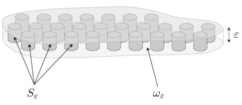
By using dimension reduction and homogenization techniques, we study the steady flow of an incompresible viscoplastic Bingham fluid in a thin porous medium. A main feature of our study is the dependence of the yield stress of the Bingham fluid on the small parameters describing the geometry of the thin porous medium under consideration. Three different problems are obtained in the limit when the small parameter $ \varepsilon $ tends to zero, following the ratio between the height $ \varepsilon $ of the porous medium and the relative dimension $ a_\varepsilon $ of its periodically distributed pores. We conclude with the interpretation of these limit problems, which all preserve the nonlinear character of the flow.
Citation: María Anguiano, Renata Bunoiu. Homogenization of Bingham flow in thin porous media[J]. Networks and Heterogeneous Media, 2020, 15(1): 87-110. doi: 10.3934/nhm.2020004
By using dimension reduction and homogenization techniques, we study the steady flow of an incompresible viscoplastic Bingham fluid in a thin porous medium. A main feature of our study is the dependence of the yield stress of the Bingham fluid on the small parameters describing the geometry of the thin porous medium under consideration. Three different problems are obtained in the limit when the small parameter $ \varepsilon $ tends to zero, following the ratio between the height $ \varepsilon $ of the porous medium and the relative dimension $ a_\varepsilon $ of its periodically distributed pores. We conclude with the interpretation of these limit problems, which all preserve the nonlinear character of the flow.

| [1] |
Darcy's laws for non-stationary viscous fluid flow in a thin porous medium. Math. Meth. Appl. Sci. (2017) 40: 2878-2895. 
|
| [2] |
On the non-stationary non-Newtonian flow through a thin porous medium. ZAMM-Z. Angew. Math. Mech. (2017) 97: 895-915.
|
| [3] |
M. Anguiano and R. Bunoiu, On the flow of a viscoplastic fluid in a thin periodic domain,, in Integral Methods in Science and Engineering (eds. C. Constanda and P. Harris), Birkhäuser, Cham, (2019), 15–24. doi: 10.1007/978-3-030-16077-7_2
|
| [4] |
M. Anguiano and F. J. Suárez-Grau, Homogenization of an incompressible non-newtonian flow through a thin porous medium,, Z. Angew. Math. Phys., 68 (2017), Art. 45, 25 pp. doi: 10.1007/s00033-017-0790-z
|
| [5] |
M. Anguiano and F. J. Suárez-Grau, The transition between the Navier-Stokes equations to the Darcy equation in a thin porous medium, Mediterr. J. Math., 15 (2018), Art. 45, 21 pp. doi: 10.1007/s00009-018-1086-z
|
| [6] |
(2013) Introduction to the Network Approximation Method for Materials Modeling. Cambridge University Press.
|
| [7] |
Homogenized non-newtonian viscoelastic rheology of a suspension of interacting particles in a viscous newtonian fluid,. SIAM Journal of Applied Mathematics (2004) 64: 1002-1034.
|
| [8] |
Laminar shallow viscoplastic fluid flowing through an array of vertical obstacles. J. Non-Newtonian Fluid Mech. (2018) 257: 59-70.
|
| [9] | D. Bresch, E. D. Fernandez-Nieto, I. Ionescu and P. Vigneaux, Augmented lagrangian method and compressible visco-plastic flows: Applications to shallow dense avalanches, in New Directions in Mathematical Fluid Mechanics. Advances in Mathematical Fluid Mechanics (eds. A.V. Fursikov, G.P. Galdi and V.V. Pukhnachev), Birkhäuser Basel, (2010), 57–89. |
| [10] | A note on homogenization of Bingham flow through a porous medium. J. Math. Pures Appl. (1993) 72: 405-414. |
| [11] |
Bingham flow in porous media with obstacles of different size. Math. Meth. Appl. Sci. (2017) 40: 4514-4528.
|
| [12] |
R. Bunoiu, G. Cardone and C. Perugia, Unfolding method for the homogenization of Bingham flow, in Modelling and Simulation in Fluid Dynamics in Porous Media. Springer Proceedings in Mathematics & Statistics (eds. J. Ferreira, S. Barbeiro, G. Pena and M. Wheeler), Vol 28, Springer, New York, NY, (2013), 109–123. doi: 10.1007/978-1-4614-5055-9_7
|
| [13] |
Asymptotic analysis of a Bingham fluid in a thin T-like shaped structure. J. Math. Pures Appl. (2019) 123: 148-166.
|
| [14] | Fluide de Bingham dans une couche mince. Annals of University of Craiova, Math. Comp. Sci. Ser. (2003) 30: 71-77. |
| [15] |
Asymptotic behaviour of a Bingham fluid in thin layers. Journal of Mathematical Analysis and Applications (2004) 293: 405-418.
|
| [16] |
The periodic unfolding method in homogenization. SIAM J. Math. Anal. (2008) 40: 1585-1620.
|
| [17] |
D. Cioranescu, A. Damlamian and G. Griso, The Periodic Unfolding Method: Theory and Applications to Partial Differential Problems, Series in Contemporary Mathematics, 3, Springer, 2018. doi: 10.1007/978-981-13-3032-2
|
| [18] |
D. Cioranescu, V. Girault and K. R. Rajagopal, Mechanics and Mathematics of Fluids of the Differential Type, Advances in Mechanics and Mathematics, 35, Springer, 2016. doi: 10.1007/978-3-319-39330-8
|
| [19] | G. Duvaut and J. L. Lions, Les Inéquations en Mécanique et en Physique, Travaux et Recherches Mathématiques, 21, Dunod, Paris, 1972. |
| [20] |
Darcy's law for flow in a periodic thin porous medium confined between two parallel plates. Transp. Porous Med. (2016) 115: 473-493.
|
| [21] |
Shallow water equations for power law and Bingham fluids. Science China Mathematics (2012) 55: 277-283.
|
| [22] |
V. Girault and P. A. Raviart, Finite Element Methods for Navier-Stokes Equations. Theory and Algorithms, Springer Series in Computational Mathematics, 5, Springer-Verlag, 1986. doi: 10.1007/978-3-642-61623-5
|
| [23] |
Asymptotic behavior of a crane. C.R.Acad.Sci. Paris, Ser. Ⅰ (2004) 338: 261-266.
|
| [24] |
Junctions between two plates and a family of beams. Math. Meth. Appl. Sci. (2018) 41: 58-79.
|
| [25] |
Asymptotic analysis for domains separated by a thin layer made of periodic vertical beams. Journal of Elasticity (2017) 128: 291-331.
|
| [26] |
Onset and dynamic shallow flow of a viscoplastic fluid on a plane slope. J. Non-Newtonian Fluid Mech. (2010) 165: 1328-1341.
|
| [27] |
Augmented lagrangian for shallow viscoplastic flow with topography. Journal of Computational Physics (2013) 242: 544-560.
|
| [28] |
Viscoplastic shallow flow equations with topography. J. Non-Newtonian Fluid Mech. (2013) 193: 116-128.
|
| [29] | Écoulement d'un fluide viscoplastique de Bingham dans un milieu poreux. J. Math. Pures Appl. (1981) 60: 341-360. |
| [30] |
P. Lipman, J. Lockwood, R. Okamura, D. Swanson and K. Yamashita, Ground Deformation Associated with the 1975 Magnitude-7.2 Earthquake and Resulting Changes in Activity of Kilauea Volcano, Hawaii, Professional Paper, 1276, Technical report, US Goverment Printing Office, 1985. doi: 10.3133/pp1276
|
| [31] |
Approximate equations for the slow spreading of a thin sheet of Bingham plastic fluid. Physics of Fluids A: Fluid Dynamics (1990) 2: 30-36.
|
| [32] |
Asymptotic analysis in elasticity problems on thin periodic structures. Networks and Heterogeneous Media (2009) 4: 577-604.
|
| [33] |
Flow of fresh concrete through steel bars: A porous medium analogy. Cement and Concrete Research (2011) 41: 496-503.
|
| [34] |
Homogenization of a stationary Navier-Stokes flow in porous medium with thin film. Acta Mathematica Scientia (2008) 28: 963-974.
|
Figures(1)
María Anguiano, Renata Bunoiu. Homogenization of Bingham flow in thin porous media[J]. Networks and Heterogeneous Media, 2020, 15(1): 87-110. doi: 10.3934/nhm.2020004


 DownLoad: