The cardiac bidomain model and homogenization

Erik Grandelius; Kenneth H. Karlsen; Erik Grandelius; Kenneth H. Karlsen

doi:10.3934/nhm.2019009

Networks and Heterogeneous Media

2019, Volume 14, Issue 1: 173-204. doi: 10.3934/nhm.2019009

Previous Article Next Article

The cardiac bidomain model and homogenization

Erik Grandelius ^,,
Kenneth H. Karlsen

Department of Mathematics, University of Oslo, P.O. Box 1053, Blindern, N–0316 Oslo, Norway

Received: 01 August 2018 Revised: 01 November 2018
Primary: 35K57, 35B27; Secondary: 35K65, 92C30

We provide a rather simple proof of a homogenization result for the bidomain model of cardiac electrophysiology. Departing from a microscopic cellular model, we apply the theory of two-scale convergence to derive the bidomain model. To allow for some relevant nonlinear membrane models, we make essential use of the boundary unfolding operator. There are several complications preventing the application of standard homogenization results, including the degenerate temporal structure of the bidomain equations and a nonlinear dynamic boundary condition on an oscillating surface.

Keywords:

Citation: Erik Grandelius, Kenneth H. Karlsen. The cardiac bidomain model and homogenization[J]. Networks and Heterogeneous Media, 2019, 14(1): 173-204. doi: 10.3934/nhm.2019009

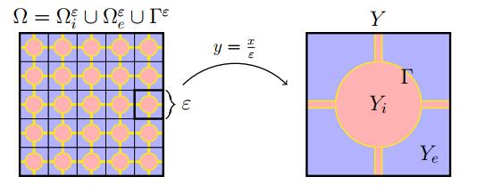
Related Papers:

[1]	Feng Qi . Completely monotonic degree of a function involving trigamma and tetragamma functions. AIMS Mathematics, 2020, 5(4): 3391-3407. doi: 10.3934/math.2020219
[2]	Wissem Jedidi, Hristo S. Sendov, Shen Shan . Classes of completely monotone and Bernstein functions defined by convexity properties of their spectral measures. AIMS Mathematics, 2024, 9(5): 11372-11395. doi: 10.3934/math.2024558
[3]	Khaled Mehrez, Abdulaziz Alenazi . Bounds for certain function related to the incomplete Fox-Wright function. AIMS Mathematics, 2024, 9(7): 19070-19088. doi: 10.3934/math.2024929
[4]	Fei Wang, Bai-Ni Guo, Feng Qi . Monotonicity and inequalities related to complete elliptic integrals of the second kind. AIMS Mathematics, 2020, 5(3): 2732-2742. doi: 10.3934/math.2020176
[5]	Xifeng Wang, Senlin Guo . Some conditions for sequences to be minimal completely monotonic. AIMS Mathematics, 2023, 8(4): 9832-9839. doi: 10.3934/math.2023496
[6]	Xi-Fan Huang, Miao-Kun Wang, Hao Shao, Yi-Fan Zhao, Yu-Ming Chu . Monotonicity properties and bounds for the complete p-elliptic integrals. AIMS Mathematics, 2020, 5(6): 7071-7086. doi: 10.3934/math.2020453
[7]	Li Xu, Lu Chen, Ti-Ren Huang . Monotonicity, convexity and inequalities involving zero-balanced Gaussian hypergeometric function. AIMS Mathematics, 2022, 7(7): 12471-12482. doi: 10.3934/math.2022692
[8]	Chuan-Yu Cai, Qiu-Ying Zhang, Ti-Ren Huang . Properties of generalized $ (p, q) $-elliptic integrals and generalized $ (p, q) $-Hersch-Pfluger distortion function. AIMS Mathematics, 2023, 8(12): 31198-31216. doi: 10.3934/math.20231597
[9]	Fei Wang, Bai-Ni Guo, Feng Qi . Correction: Monotonicity and inequalities related to complete elliptic integrals of the second kind. AIMS Mathematics, 2020, 5(6): 5683-5684. doi: 10.3934/math.2020363
[10]	Moquddsa Zahra, Dina Abuzaid, Ghulam Farid, Kamsing Nonlaopon . On Hadamard inequalities for refined convex functions via strictly monotone functions. AIMS Mathematics, 2022, 7(11): 20043-20057. doi: 10.3934/math.20221096

Abstract

1. Introduction

It is well known that the convexity ^{[1,2,3,4,5,6,8,9,11,15,16,40,55,63,64]}, monotonicity ^{[7,12,13,14,41,42,43,44,45,46,47,48,49,50,51,52,53]} and complete monotonicity ^{[58,59,61,62]} have widely applications in many branches of pure and applied mathematics ^{[19,24,28,32,35,38,65]}. In particular, many important inequalities ^{[20,25,30,33,37,39,69]} can be discovered by use of the convexity, monotonicity and complete monotonicity. The concept of complete monotonicity can be traced back to 1920s ^[18]. Recently, the complete monotonicity has attracted the attention of many researchers ^{[23,34,56,67]} due to it has become an important tool to study geometric function theory ^[26,31,36], its definition can be simply stated as follows.

Definition 1.1. Let $ I\subseteq \mathbb{R} $ be an interval. Then a real-valued function $ f: I\mapsto\mathbb{R} $ is said to be completely monotonic on $ I $ if $ f $ has derivatives of all orders on $ I $ and satisfies

$\begin{equation} (-1)^{n}f^{(n)}(x)\geq 0 \end{equation}$ $

(1.1)

for all $ x\in I $ and $ n = 0, 1, 2, \cdots $.

If $ I = (0, \infty) $, then a necessary and sufficient condition for the complete monotonicity can be found in the literature ^[54]: the real-valued function $ f: (0, \infty)\mapsto\mathbb{R} $ is completely monotonic on $ (0, \infty) $ if and only if

$\begin{equation} f\left(x\right) = \int_{0}^{\infty }e^{-xt}d\alpha \left(t\right) \end{equation}$ $

(1.2)

is a Laplace transform, where $ \alpha\left(t\right) $ is non-decreasing and such that the integral of (1.2) converges for $ 0 < x < \infty $.

In 1997, Alzer ^[10] studied a class of completely monotonic functions involving the classical Euler gamma function ^{[21,22,60,66,68]} and obtained the following result.

Theorem 1.1. Let $ n\geq 0 $ be an integer, $ \kappa(x) $ and $ f_{n}\left(x\right) $ be defined on $ (0, \infty) $ by

$\begin{equation} \kappa(x) = \ln\Gamma\left(x\right)-\left(x-\dfrac{1}{2}\right)\ln x+x-\dfrac{1 }{2}\ln\left(2\pi\right) \end{equation}$ $

(1.3)

and

$\begin{equation} f_{n}\left( x\right) = \left\{ \begin{array}{ll} \kappa (x)-\sum\limits_{k = 1}^{n}\frac{B_{2k}}{2k\left( 2k-1\right) x^{2k-1}}, & n\geq 1, \\ \kappa (x), & n = 0, \end{array} \right. \end{equation}$ $

(1.4)

where $ B_{n} $ denotes the Bernoulli number. Then both the functions $ x\mapsto f_{2n}\left(x\right) $ and $ x\mapsto -f_{2n+1}\left(x\right) $ are strictly completely monotonic on $ \left(0, \infty \right) $.

In 2009, Koumandos and Pedersen ^[27] first introduced the concept of completely monotonic functions of order $ r $. In 2012, Guo and Qi ^[17] proposed the concept of completely monotonic degree of nonnegative functions on $ (0, \infty) $. Since the completely monotonic degrees of many functions are integers, in this paper we introduce the concept of the completely monotonic integer degree as follows.

Definition 1.2. Let $ f(x) $ be a completely monotonic function on $ (0, \infty) $ and denote $ f(\infty) = \lim_{x\rightarrow \infty }f(x) $. If there is a most non-negative integer $ k $ $ (\leq \infty) $ such that the function $ x^{k}[f(x)-f(\infty)] $ is completely monotonic on $ (0, \infty) $, then $ k $ is called the completely monotonic integer degree of $ f(x) $ and denoted as $ \deg _{cmi}^{x}\left[f\left(x\right) \right] = k $.

Recently, Qi and Liu ^[29] gave a number of conjectures about the completely monotonic degrees of these fairly broad classes of functions. Based on thirty six figures of the completely monotonic degrees, the following conjectures for the functions $ \left(-1\right) ^{m}R_{n}^{(m)}(x) = \left(-1\right) ^{m}\left[\left(-1\right) ^{n}f_{n}(x) \right] ^{\left(m\right) } = \left(-1\right) ^{m+n}f_{n}^{\left(m\right) }(x) $ are shown in ^[29]:

(ⅰ) If $ m = 0, $ then

$\begin{equation} \deg _{cmi}^{x}\left[ R_{n}(x)\right] = \left\{ \begin{array}{cc} 0, & \text{if }n = 0 \\ 1, & \text{if }n = 1 \\ 2\left( n-1\right) , & \text{if }n\geq 2 \end{array} \right.; \end{equation}$ $

(1.5)

(ⅱ) If $ m = 1 $, then

$\begin{equation} \deg _{cmi}^{x}\left[ -R_{n}^{\prime }(x)\right] = \left\{ \begin{array}{cc} 1, & \text{if }n = 0 \\ 2, & \text{if }n = 1 \\ 2n-1, & \text{if }n\geq 2 \end{array} \right.; \end{equation}$ $

(1.6)

(ⅲ) If $ m\geq 1, $ then

$\begin{equation} \deg _{cmi}^{x}\left[ \left( -1\right) ^{m}R_{n}^{\left( m\right) }(x)\right] = \left\{ \begin{array}{cc} m-1, & \text{if }n = 0 \\ m, & \text{if }n = 1 \\ m+2\left( n-1\right) , & \text{if }n\geq 2 \end{array} \right. . \end{equation}$ $

(1.7)

In this paper, we get the complete monotonicity of lower-order derivative and lower-scalar functions $ \left(-1\right) ^{m}R_{n}^{(m)}(x) $ and their completely monotonic integer degrees using the Definition 1.2 and a common sense in Laplace transform that the original function has the one-to-one correspondence with the image function, and demonstrated the correctness of the existing conjectures by using a elementary simple method. The negative conclusion to the second clause of (1.7) is given. Finally, we propose some operational conjectures which involve the completely monotonic integer degrees for the functions $ \left(-1\right) ^{m}R_{n}^{(m)}(x) $ for $ m = 0, 1, 2, \cdots $.

2. Lemmas

In order to prove our main results, we need several lemmas and a corollary which we present in this section.

Lemma 2.1. If the function $ x^{n}f(x) $ $ (n\geq 1) $ is completely monotonic on $ (0, \infty) $, so is the function $ x^{n-1}f(x) $.

Proof. Since the function $ 1/x $ is completely monotonic on $ (0, \infty) $, we have $ x^{n-1}f(x) = \left(1/x\right) \left[x^{n}f(x)\right] $ is completely monotonic on $ (0, \infty) $ too.

Corollary 2.1. Let $ \alpha \left(t\right) \geq 0 $ be given in (1.2). Then the functions $ x^{i-1}f(x) $ for $ i = n, n-1, \cdots, 2, 1 $ are completely monotonic on $ (0, \infty) $ if the function $ x^{n}f(x) $ $ (n\in \mathbb{N}) $ is completely monotonic on $ (0, \infty) $.

The above Corollary 2.1 is a theoretical cornerstone to find the completely monotonic integer degree of a function $ f(x) $. According to this theory and Definition 1.2, we only need to find a nonnegative integer $ k $ such that $ x^{k}f(x) $ is completely monotonic on $ (0, \infty) $ and $ x^{k+1}f(x) $ is not, then $ \deg _{cmi}^{x}\left[f(x)\right] = k $.

The following lemma comes from Yang ^[57]:

Lemma 2.2. Let $ f_{n}\left(x\right) $ be defined as (1.4). Then $ f_{n}\left(x\right) $ can be written as

$\begin{equation} f_{n}\left( x\right) = \frac{1}{4}\int_{0}^{\infty }p_{n}\left( \frac{t}{2} \right) e^{-xt}dt, \end{equation}$ $

(2.1)

where

$\begin{equation} p_{n}\left( t\right) = \frac{\coth t}{t}-\sum\limits_{k = 0}^{n}\frac{2^{2k}B_{2k}}{ \left( 2k\right) !}t^{2k-2}. \end{equation}$ $

(2.2)

Lemma 2.3. Let $ m, r\geq 0, $ $ n\geq 1, $ $ f_{n}\left(x\right) $ and $ p_{n}\left(t\right) $ be defined as (2.1) and (2.2). Then

$\begin{equation} x^{r}\left( -1\right) ^{m}R_{n}^{\left( m\right) }(x) = x^{r}\left( -1\right) ^{m+n}f_{n}^{\left( m\right) }(x) = \frac{1}{4}\int_{0}^{\infty }\left[ \left( -1\right) ^{n}t^{m}p_{n}\left( \frac{t}{2}\right) \right] ^{(r)}e^{-xt}dt. \end{equation}$ $

(2.3)

Proof. It follows from (2.1) that

$\begin{eqnarray*} x\left( -1\right) ^{m}R_{n}^{\left( m\right) }(x) & = &x\left( -1\right) ^{m+n}f_{n}^{\left( m\right) }(x) = x\left( -1\right) ^{m+n}\frac{1}{4} \int_{0}^{\infty }\left( -t\right) ^{m}p_{n}\left( \frac{t}{2}\right) e^{-xt}dt \\ & = &x\left( -1\right) ^{n}\frac{1}{4}\int_{0}^{\infty }t^{m}p_{n}\left( \frac{ t}{2}\right) e^{-xt}dt = \left( -1\right) ^{n-1}\frac{1}{4}\int_{0}^{\infty }t^{m}p_{n}\left( \frac{t}{2}\right) de^{-xt} \\ & = &\left( -1\right) ^{n-1}\frac{1}{4}\left\{ \left[ t^{m}p_{n}\left( \frac{t }{2}\right) e^{-xt}\right] _{t = 0}^{\infty }-\int_{0}^{\infty }\left[ t^{m}p_{n}\left( \frac{t}{2}\right) \right] ^{\prime }e^{-xt}dt\right\} \\ & = &\left( -1\right) ^{n}\frac{1}{4}\int_{0}^{\infty }\left[ t^{m}p_{n}\left( \frac{t}{2}\right) \right] ^{\prime }e^{-xt}dt. \end{eqnarray*}$ $

Repeat above process. Then we come to the conclusion that

$\begin{equation*} x^{r}\left( -1\right) ^{m}R_{n}^{\left( m\right) }(x) = \left( -1\right) ^{n} \frac{1}{4}\int_{0}^{\infty }\left[ t^{m}p_{n}\left( \frac{t}{2}\right) \right] ^{(r)}e^{-xt}dt, \end{equation*}$ $

which completes the proof of Lemma 2.3.

3. Complete monotonicity of the functions $ R_{n}(x) $ and their completely monotonic integer degrees

In recent paper ^[70] the reslut $ \deg _{cmi}^{x}\left[R_{1}(x)\right] = \deg _{cmi}^{x}\left[-f_{1}\left(x\right) \right] = 1 $ was proved. In this section, we mainly discuss $ \deg _{cmi}^{x}\left[R_{2}(x)\right] $ and $ \deg _{cmi}^{x}\left[R_{3}(x)\right] $. Then discuss whether the most general conclusion exists about $ \deg _{cmi}^{x}\left[R_{n}(x)\right] $.

Theorem 3.1. The function $ x^{3}R_{2}(x) $ is not completely monotonic on $ \left(0, \infty \right) $, and

$ \deg _{cmi}^{x}\left[ R_{2}(x)\right] = \deg _{cmi}^{x}\left[ f_{2}\left( x\right) \right] = 2. $

Proof. Note that the function $ x^{2}R_{2}(x) $ is completely monotonic on $ (0, \infty) $ due to

$\begin{eqnarray*} x^{2}R_{2}(x) & = &\frac{1}{4}\int_{0}^{\infty }p_{2}^{(2)}\left( \frac{t}{2} \right) e^{-xt}dt, \\ p_{2}\left( t\right) & = & \frac{\coth t}{t}+\frac{1}{45}t^{2}- \frac{1}{t^{2}}-\frac{1}{3}, \\ p_{2}^{\prime }\left( t\right) & = & \frac{2}{45}t-\frac{1}{t\sinh ^{2}t}+\frac{2}{t^{3}}-\frac{1}{t^{2}}\frac{\cosh t}{\sinh t}, \\ p_{2}^{\prime \prime }\left( t\right) & = &\frac{45A(t)+180t^{2}B(t)+t^{4}C(t) }{90t^{4}\sinh ^{3}t} \gt 0, \end{eqnarray*}$ $

where

$\begin{eqnarray*} A(t) & = &t\cosh 3t-3\sinh 3t+9\sinh t-t\cosh t \\ & = &\sum\limits_{n = 5}^{\infty }\frac{2\left( n-4\right) \left( 3^{2n}-1\right) }{ \left( 2n+1\right) !}t^{2n+1} \gt 0, \\ B(t) & = &t\cosh t+\sinh t \gt 0, \\ C(t) & = &\sinh 3t-3\sinh t \gt 0. \end{eqnarray*}$ $

So $ \deg _{cmi}^{x}\left[R_{2}(x)\right] \geq 2 $.

On the other hand, we can prove that the function $ x^{3}f_{2}\left(x\right) = x^{3}R_{2}(x) $ is not completely monotonic on $ (0, \infty) $. By (2.3) we have

$\begin{equation*} x^{3}f_{2}\left( x\right) = \frac{1}{4}\int_{0}^{\infty }p_{2}^{(3)}\left( \frac{t}{2}\right) e^{-xt}dt, \end{equation*}$ $

then by (1.2), we can complete the staged argument since we can verify

$\begin{equation*} p_{2}^{(3)}\left( \frac{t}{2}\right) \gt 0\Longleftrightarrow p_{2}^{(3)}\left( t\right) \gt 0 \end{equation*}$ $

is not true for all $ t > 0 $ due to

$\begin{eqnarray*} p_{2}^{\prime \prime \prime }\left( t\right) & = &\frac{2}{t\sinh ^{2}t}-\frac{ 2}{t^{3}\sinh ^{2}t}+\frac{4}{t^{3}}+\frac{24}{t^{5}}-\frac{6}{t}\frac{\cosh ^{2}t}{\sinh ^{4}t}-\frac{4}{t^{3}}\frac{\cosh ^{2}t}{\sinh ^{2}t}-\frac{2}{ t^{2}}\frac{\cosh ^{3}t}{\sinh ^{3}t} \\ &&+\frac{2}{t^{2}}\frac{\cosh t}{\sinh t}-\frac{4}{t^{2}}\frac{\cosh t}{ \sinh ^{3}t}-\frac{6}{t^{4}}\frac{\cosh t}{\sinh t} \end{eqnarray*}$ $

with $ p_{2}^{\prime \prime \prime }\left(10\right) = -0.000\, 36\cdots $.

Theorem 3.2. The function $ x^{4}R_{3}(x) $ is completely monotonic on $ \left(0, \infty \right) $, and

$ \deg _{cmi}^{x}\left[ R_{3}(x)\right] = \deg _{cmi}^{x}\left[ -f_{3}\left( x\right) \right] = 4. $

Proof. By (2.3) we obtain that

$\begin{equation*} x^{4}R_{3}(x) = \int_{0}^{\infty }\left[ -p_{3}^{(4)}\left( \frac{t}{2}\right) \right] e^{-xt}dt. \end{equation*}$ $

From (2.2) we clearly see that

$\begin{equation*} p_{3}\left( t\right) = \frac{\coth t}{t}-\frac{1}{t^{2}}+\frac{1}{ 45}t^{2}-\frac{2}{945}t^{4}-\frac{1}{3}, \end{equation*}$ $

$\begin{equation*} p_{3}^{(4)}\left( t\right) = :- \frac{1}{630}\frac{H(t)}{ t^{6}\sinh ^{5}t} , \end{equation*}$ $

$\begin{equation*} -p_{3}^{(4)}\left( t\right) = \frac{1}{630}\frac{H(t)}{t^{6}\sinh ^{5}t} , \end{equation*}$ $

where

$\begin{eqnarray*} H(t) & = &\left( 2t^{6}+4725\right) \sinh 5t- 945t\cosh 5t-\left( 1260t^{5}+ 3780t^{3}-2835t\right) \cosh 3t \\ &&-\left( 10t^{6}+2520t^{4}+3780t^{2} +23\, 625\right) \sinh 3t-\left( 13\, 860t^{5}-3780t^{3}+1890t\right) \cosh t \\ &&+\left( 20t^{6}-7560t^{4}+ 11\, 340t^{2}+47\, 250\right) \sinh t \\ &:& = \sum\limits_{n = 5}^{\infty }\frac{h_{n}}{\left( 2n+3\right) !}t^{2n+3} \end{eqnarray*}$ $

with

$\begin{eqnarray*} h_{n} & = & \frac{2}{125}\left[ 64n^{6}+96n^{5}-80n^{4}-120n^{3}+16n^{2}-2953\, 101n+32\, 484\, 375\right] 5^{2n} \\ &&-\frac{10}{27}\left[ 64n^{6}+96n^{5}+5968n^{4}+105\, 720n^{3}+393 \, 136n^{2}+400\, 515n+1760\, 535\right] 3^{2n} \\ &&+20\left[ 64n^{6}+96n^{5}-11\, 168n^{4}-9696n^{3}+9592n^{2}+13\, 191n+7749 \right] \\ & \gt &0 \end{eqnarray*}$ $

for all $ n\geq 5 $. So $ x^{4}R_{3}(x) $ is completely monotonic on $ (0, \infty) $, which implies $ \deg _{cmi}^{x}\left[R_{3}(x)\right] \geq 4 $.

Then we shall prove $ x^{5}R_{3}(x) = -x^{5}f_{3}\left(x\right) $ is not completely monotonic on $ (0, \infty) $. Since

$\begin{equation*} x^{5}R_{3}(x) = \int_{0}^{\infty }\left[ -p_{3}^{(5)}\left( \frac{t}{2}\right) \right] e^{-xt}dt, \end{equation*}$ $

and

$\begin{equation*} -p_{3}^{(5)}\left( t\right) = \frac{ 1}{4}\frac{K(t)}{t^{7}\sinh ^{6}t}, \end{equation*}$ $

where

$\begin{eqnarray*} K(t) & = &540\cosh 4t-1350\cosh 2t-90\cosh 6t-240t^{2}\cosh 2t+60t^{2}\cosh 4t \\ &&+80t^{4}\cosh 2t+40t^{4}\cosh 4t+208t^{6}\cosh 2t+8t^{6}\cosh 4t-120t^{3}\sinh 2t \\ &&+60t^{3}\sinh 4t+200t^{5}\sinh 2t+20t^{5}\sinh 4t+75t\sinh 2t-60t\sinh 4t \\ &&+15t\sinh 6t+180t^{2}-120t^{4}+264t^{6}+900. \end{eqnarray*}$ $

We find $ K(5)\thickapprox -2.\, 631\, 5\times 10^{13} < 0 $, which means $ -p_{3}^{(5)}\left(5\right) < 0 $. So the function $ x^{5}R_{3}(x) = -x^{5}f_{3}\left(x\right) $ is not completely monotonic on $ (0, \infty) $.

In a word, $ \deg _{cmi}^{x}\left[R_{3}(x)\right] = \deg _{cmi}^{x}\left[-f_{3}\left(x\right) \right] = 4. $

Remark 3.1. So far, we have the results about the completely monotonic integer degrees of such functions, that is, $ \deg _{cmi}^{x}\left[R_{1}(x)\right] = 1 $ and $ \deg _{cmi}^{x}\left[R_{n}(x) \right] = 2\left(n-1\right) $ for $ n = 2, 3 $, and find that the existing conclusions support the conjecture (1.5).

4. Complete monotonicity of the functions $ -R_{n}^{\prime }(x) $ $ ($ $ 1\leq n\leq 3) $ and their completely monotonic integer degrees

In this section, we shall calculate the completely monotonic degrees of the functions $ \left(-1\right) ^{m}R_{n}^{(m)}(x) $, where $ m = 1 $ and $ 1\leq n\leq 3. $

Theorem 4.1 The function $ -x^{2}R_{1}^{\prime }(x) = x^{2}f_{1}^{\prime }(x) $ is completely monotonic on $ \left(0, \infty \right) $, and

$ \deg _{cmi}^{x}\left[ \left( -1\right) ^{1}R_{1}^{\prime }(x)\right] = 2. $

Proof. By the integral representation (2.3) we obtain

$\begin{equation*} x^{2}f_{1}^{\prime }\left( x\right) = \frac{1}{4}\int_{0}^{\infty }\left[ -tp_{1}\left( \frac{t}{2}\right) \right] ^{\prime \prime }e^{-xt}dt. \end{equation*}$ $

So we complete the proof of result that $ x^{2}f_{1}^{\prime }(x) $ is completely monotonic on $ \left(0, \infty \right) $ when proving

$\begin{equation*} \left[ -tp_{1}\left( \frac{t}{2}\right) \right] ^{\prime \prime } \gt 0\Longleftrightarrow \left[ tp_{1}\left( \frac{t}{2}\right) \right] ^{\prime \prime } \lt 0\Longleftrightarrow \left[ tp_{1}\left( t\right) \right] ^{\prime \prime } \lt 0. \end{equation*}$ $

In fact,

$\begin{eqnarray*} tp_{1}\left( t\right) & = &t\left( \frac{\coth t}{t}-\frac{1}{t^{2}}-\frac{1}{3 }\right) = \frac{\cosh t}{\sinh t}-\frac{1}{3}t-\frac{1}{t}, \\ \left[ tp_{1}\left( t\right) \right] ^{\prime } & = & \frac{1}{t^{2} }-\frac{\cosh ^{2}t}{\sinh ^{2}t}+\frac{2}{3}, \\ \left[ tp_{1}\left( t\right) \right] ^{\prime \prime } & = &\frac{2}{\sinh ^{3}t}\left[ \cosh t-\left( \frac{\sinh t}{t}\right) ^{3}\right] \lt 0. \end{eqnarray*}$ $

Then we have $ \deg _{cmi}^{x}\left[\left(-1\right) ^{1}R_{1}^{\prime }(x)] \right. \geq 2. $

Here $ -x^{3}R_{1}^{\prime }(x) = x^{3}f_{1}^{\prime }(x) $ is not completely monotonic on $ \left(0, \infty \right) $. By (2.2) and (2.3) we have

$\begin{equation*} x^{3}f_{1}^{\prime }\left( x\right) = \frac{1}{4}\int_{0}^{\infty }\left[ -tp_{1}\left( \frac{t}{2}\right) \right] ^{\prime \prime \prime }e^{-xt}dt, \end{equation*}$ $

and

$\begin{equation*} \left[ -tp_{1}\left( t\right) \right] ^{\prime \prime \prime } = 2\frac{ 3t^{4}\cosh ^{2}t-t^{4}\sinh ^{2}t-3\sinh ^{4}t}{t^{4}\sinh ^{4}t} \end{equation*}$ $

with $ \left[-tp_{1}\left(t\right) \right] ^{\prime \prime \prime }\left\vert _{t = 2}\right. \thickapprox -3.\, 623\, 7\times 10^{-2} < 0. $

Theorem 4.2. The function $ -x^{3}R_{2}^{\prime }(x) $ is completely monotonic on $ \left(0, \infty \right) $, and

$ \deg _{cmi}^{x}\left[ -R_{2}^{\prime }(x)\right] = \deg _{cmi}^{x}\left[ -f_{2}^{\prime }(x)\right] = 3. $

Proof. First, we can prove that the function $ -x^{3}R_{2}^{\prime }(x) $ is completely monotonic on $ \left(0, \infty \right) $. Using the integral representation (2.3) we obtain

$\begin{equation*} -x^{3}f_{2}^{\prime }\left( x\right) = \frac{1}{4}\int_{0}^{\infty }\left[ tp_{2}\left( \frac{t}{2}\right) \right] ^{(3)}e^{-xt}dt, \end{equation*}$ $

and complete the proof of the staged argument when proving

$\begin{equation*} \left[ tp_{2}\left( \frac{t}{2}\right) \right] ^{(3)} \gt 0\Longleftrightarrow \left[ tp_{2}\left( t\right) \right] ^{(3)} \gt 0. \end{equation*}$ $

In fact,

$\begin{eqnarray*} p_{2}\left( t\right) & = & \frac{\coth t}{t}+\frac{1}{45}t^{2}- \frac{1}{t^{2}}-\frac{1}{3}, \\ L(t) &:& = tp_{2}\left( t\right) = \frac{\cosh t}{\sinh t}-\frac{1}{3}t-\frac{1 }{t}+\frac{1}{45}t^{3}, \end{eqnarray*}$ $

$\begin{eqnarray*} L^{\prime \prime \prime }(t) & = &\frac{-180\cosh 2t+45\cosh 4t-124t^{4}\cosh 2t+t^{4}\cosh 4t-237t^{4}+135}{60t^{4}\sinh ^{4}t} \\ & = &\frac{1}{60t^{4}\sinh ^{4}t}\left[ \sum\limits_{n = 3}^{\infty }\frac{ 2^{2n+2}b_{n} }{\left( 2n+4\right) !}t^{2n+4}\right] \gt 0, \end{eqnarray*}$ $

where

$\begin{eqnarray*} b_{n} & = &2^{2n}\left( 4n^{4}+20n^{3}+35n^{2}+25n+2886\right) \\ &&-4\left( 775n+1085n^{2}+620n^{3}+124n^{4}+366\right) \\ & \gt &0 \end{eqnarray*}$ $

for all $ n\geq 3 $.

On the other hand, by (2.3) we obtain

$\begin{equation*} x^{4}\left( -1\right) ^{1}R_{2}^{\prime}(x) = -x^{4}f_{2}^{\prime }\left( x\right) = \frac{1}{4}\int_{0}^{\infty }\left[ tp_{2}\left( \frac{t}{2 }\right) \right] ^{(4)}e^{-xt}dt, \end{equation*}$ $

and

$\begin{equation*} L^{(4)}(t) = \left[ tp_{2}\left( t\right) \right] ^{(4)} = 16\frac{\cosh t}{ \sinh t}-40\frac{\cosh ^{3}t}{\sinh ^{3}t}+24\frac{\cosh ^{5}t}{\sinh ^{5}t}- \frac{24}{t^{5}} \end{equation*}$ $

is not positive on $ \left(0, \infty \right) $ due to $ L^{(4)}(10) \thickapprox -2.\, 399\, 3\times 10^{-4} < 0 $, we have that $ -x^{4}R_{2}^{\prime }(x) $ is not completely monotonic on $ \left(0, \infty \right) $.

Theorem 4.3. The function $ -x^{5}R_{3}^{\prime }(x) $ is completely monotonic on $ \left(0, \infty \right) $, and

$ \deg _{cmi}^{x}\left[ -R_{3}^{\prime }(x)\right] = \deg _{cmi}^{x}\left[ f_{3}^{\prime }(x)\right] = 5. $

Proof. We shall prove that $ -x^{5}R_{3}^{\prime }(x) = x^{5}f_{3}^{\prime }(x) $ is completely monotonic on $ \left(0, \infty \right) $ and $ -x^{6}R_{3}^{\prime }(x) = x^{6}f_{3}(x) $ is not. By (2.2) and (2.3) we obtain

$\begin{equation*} x^{r}f_{3}^{\prime }(x) = \frac{1}{4}\int_{0}^{\infty }\left[ -tp_{3}\left( \frac{t}{2}\right) \right] ^{(r)}e^{-xt}dt, \text{ }r\geq 0. \end{equation*}$ $

and

$\begin{eqnarray*} p_{3}\left( t\right) & = & \frac{\coth t}{t}-\frac{1}{t^{2}}+\frac{1 }{45}t^{2}-\frac{2}{945}t^{4}-\frac{1}{3}, \\ M(t) &:& = tp_{3}\left( t\right) = \frac{\cosh t}{\sinh t}-\frac{1}{3}t-\frac{1 }{t}+\frac{1}{45}t^{3}-\frac{2}{945}t^{5}, \\ M^{(5)}(t) & = &-\frac{1}{252}\frac{p(t)}{t^{6}\sinh ^{6}t}, \end{eqnarray*}$ $

we have

$\begin{eqnarray*} \left[ -M(t)\right] ^{(5)} & = &\frac{1}{252}\frac{p(t)}{t^{6}\sinh ^{6}t}, \\ \left[ -M(t)\right] ^{(6)} & = & \frac{1}{4}\frac{q(t)}{t^{7}\sinh ^{7}t}, \end{eqnarray*}$ $

where

$\begin{eqnarray*} p(t) & = &-14\, 175\cosh 2t+5670\cosh 4t-945\cosh 6t+13\, 134t^{6}\cosh 2t \\ &&+492t^{6}\cosh 4t+2t^{6}\cosh 6t+16\, 612t^{6}+9450, \\ q(t) & = & 945\sinh 3t-315\sinh 5t+45\sinh 7t-1575 \sinh t-456t^{7}\cosh 3t \\ &&-8t^{7}\cosh 5t-2416 t^{7}\cosh t. \end{eqnarray*}$ $

Since

$\begin{eqnarray*} p(t) & = &\sum\limits_{n = 4}^{\infty }\frac{2\cdot 6^{2n}+492\cdot 4^{2n}+ 13\, 134\cdot 2^{2n}}{\left( 2n\right) !}t^{2n+6} \\ &&-\sum\limits_{n = 4}^{\infty }\frac{945\cdot 6^{2n+6}-5670\cdot 4^{2n+6}+14\, 175\cdot 2^{2n+6}}{\left( 2n+6\right) !}t^{2n+6} \\ & \gt &0, \\ q(0.1) &\thickapprox &-2.9625\times 10^{-5} \lt 0, \end{eqnarray*}$ $

we obtain the expected conclusions.

Remark 4.1. The experimental results show that the conjecture (1.6) may be true.

5. Complete monotonicity of the functions $ R_{n}^{\prime \prime }(x) $ $ ($ $ 1\leq n\leq 3) $ and their completely monotonic integer degrees

Theorem 5.1. The function $ x^{3}R_{1}^{\prime \prime }(x) $ is completely monotonic on $ \left(0, \infty \right) $, and

$\begin{equation} \deg _{cmi}^{x}\left[ R_{1}^{\prime \prime }(x)\right] = \deg _{cmi}^{x}\left[ -f_{1}^{\prime \prime }(x)\right] = 3. \end{equation}$ $

(5.1)

Proof. By (2.2) and (2.3) we obtain

$\begin{equation*} x^{3}R_{1}^{\prime \prime }(x) = -x^{3}f_{1}^{\prime \prime }(x) = \frac{1}{4} \int_{0}^{\infty }\left[ -t^{2}p_{1}\left( \frac{t}{2}\right) \right] ^{\prime \prime \prime }e^{-xt}dt, \end{equation*}$ $

and

$\begin{equation*} t^{2}p_{1}\left( t\right) = t\frac{\cosh t}{\sinh t}-\frac{1}{3} t^{2}-1, \end{equation*}$ $

$\begin{equation*} \left[ -t^{2}p_{1}\left( t\right) \right] ^{\prime \prime \prime } = \frac{2}{3\sinh ^{4}t}\left[ \sum\limits_{n = 2}^{\infty } \frac{3\left( n-1\right) 2^{2n+1}}{\left( 2n+1\right) !}t^{2n+1}\right] \gt 0. \end{equation*}$ $

So $ x^{3}R_{1}^{\prime \prime }(x) $ is completely monotonic on $ \left(0, \infty \right) $.

But $ x^{4}R_{1}^{\prime \prime }(x) $ is not completely monotonic on $ \left(0, \infty \right) $ due to

$\begin{equation*} x^{4}R_{1}^{\prime \prime }(x) = \frac{1}{4}\int_{0}^{\infty }\left[ -t^{2}p_{1}\left( \frac{t}{2}\right) \right] ^{(4)}e^{-xt}dt, \end{equation*}$ $

and

$\begin{equation*} \left[ -t^{2}p_{1}\left( t\right) \right] ^{(4)} = \frac{1}{\sinh ^{5}t}\left( 4\sinh 3t+12\sinh t-22t\cosh t-2t\cosh 3t\right) \end{equation*}$ $

with $ \left[-t^{2}p_{1}\left(t\right) \right] ^{(4)}\vert _{t = 10}\thickapprox -5.\, 276\, 6\times 10^{-7} < 0. $

$\begin{equation*} \deg _{cmi}^{x}\left[ R_{1}^{\prime \prime }(x)\right] = \deg _{cmi}^{x}\left[ -f_{1}^{\prime \prime }(x)\right] = 3. \end{equation*}$ $

Remark 5.1. Here, we actually give a negative answer to the second paragraph of conjecture (1.7).

Theorem 5.2. The function $ x^{4}R_{2}^{\prime \prime }(x) $ is completely monotonic on $ \left(0, \infty \right) $, and

$ \deg _{cmi}^{x}\left[ R_{2}^{\prime \prime }(x)\right] = \deg _{cmi}^{x}\left[ f_{2}^{\prime \prime }(x)\right] = 4. $

Proof. By (2.2) and (2.3) we

$\begin{equation*} x^{4}f_{2}^{\prime \prime }(x) = \frac{1}{4}\int_{0}^{\infty }\left[ t^{2}p_{2}\left( \frac{t}{2}\right) \right] ^{(4)}e^{-xt}dt, \end{equation*}$ $

and

$\begin{eqnarray*} t^{2}p_{2}\left( t\right) & = & \frac{1}{45}t^{4}-\frac{1}{3}t^{2}+t \frac{\cosh t}{\sinh t}-1, \\ \left[ t^{2}p_{2}\left( t\right) \right] ^{(4)} & = &\frac{1}{30}\frac{\left( -125\sinh 3t+\sinh 5t-350\sinh t+660t\cosh t+60t\cosh 3t\right) }{\sinh ^{5}t} \\ & = &\frac{1}{30\sinh ^{5}t}\left[ \sum\limits_{n = 3}^{\infty }\frac{5\left( 5^{2n}+\left( 24n-63\right) 3^{2n}+264n+62\right) }{\left( 2n+1\right) !} t^{2n+1}\right] \\ & \gt &0. \end{eqnarray*}$ $

Since

$\begin{equation*} x^{5}f_{2}^{\prime \prime }(x) = \frac{1}{4}\int_{0}^{\infty }\left[ t^{2}p_{2}\left( \frac{t}{2}\right) \right] ^{(5)}e^{-xt}dt, \end{equation*}$ $

and

$\begin{equation*} \left[ t^{2}p_{2}\left( t\right) \right] ^{(5)} = \frac{ 50\sinh 2t-66t+5\sinh 4t-52t\cosh 2t- 2t\cosh 4t}{\sinh ^{6}t} \end{equation*}$ $

with $ \left[t^{2}p_{2}\left(t\right) \right] ^{(5)}\left\vert _{t = 10}\right. \thickapprox -9.\, 893\, 5\times 10^{-7} < 0 $, we have that $ x^{5}f_{2}^{\prime \prime }(x) $ is not completely monotonic on $ \left(0, \infty \right) $. So

$\begin{equation*} \deg _{cmi}^{x}\left[ R_{2}^{\prime \prime }(x)\right] = 4. \end{equation*}$ $

Theorem 5.3. The function $ x^{6}R_{3}^{\prime \prime }(x) $ is completely monotonic on $ \left(0, \infty \right) $, and

$ \deg _{cmi}^{x}\left[ R_{3}^{\prime \prime }(x)\right] = \deg _{cmi}^{x}\left[ -f_{3}^{\prime \prime }(x)\right] = 6. $

Proof. By the integral representation (2.3) we obtain

$\begin{eqnarray*} -x^{6}f_{3}^{\prime \prime }(x) & = &\frac{1}{4}\int_{0}^{\infty }\left[ -t^{2}p_{3}\left( \frac{t}{2}\right) \right] ^{(6)}e^{-xt}dt, \\ -x^{7}f_{3}^{\prime \prime }(x) & = &\frac{1}{4}\int_{0}^{\infty }\left[ -t^{2}p_{3}\left( \frac{t}{2}\right) \right] ^{(7)}e^{-xt}dt. \end{eqnarray*}$ $

It follows from (2.2) that

$\begin{eqnarray*} p_{3}\left( t\right) & = & \frac{\coth t}{t}-\frac{1}{t^{2}}+\frac{1 }{45}t^{2}-\frac{2}{945}t^{4}-\frac{1}{3}, \\ N(t) &:& = t^{2}p_{3}\left( t\right) = \frac{1}{45}t^{4}-\frac{1}{3} t^{2}-\frac{2}{945}t^{6}+t\frac{\cosh t}{\sinh t}-1, \\ -N^{(6)}(t) & = &\frac{1}{42}\frac{r(t)}{\sinh ^{7}t} , \\ -N^{(7)}(t) & = & \frac{\left( \begin{array}{c} 2416t-1715\sinh 2t-392\sinh 4t-7\sinh 6t \\ +2382t\cosh 2t+240t\cosh 4t+2t\cosh 6t \end{array} \right) }{\sinh ^{8}t}, \end{eqnarray*}$ $

where

$\begin{eqnarray*} r(t) & = & 6321\sinh 3t+245\sinh 5t+\sinh 7t+10\, 045 \sinh t-25\, 368t\cosh t \\ &&-4788t\cosh 3t-84 t\cosh 5t \\ & = &\sum\limits_{n = 4}^{\infty }\frac{c_{n}}{\left( 2n+1\right) !}t^{2n+1} \end{eqnarray*}$ $

with

$\begin{equation*} c_{n} = 7\cdot 7^{2n}-\left( 168n-1141\right) 5^{2n}-\left( 9576n-14\, 175\right) 3^{2n}-\left( 50\, 736n+15\, 323\right) . \end{equation*}$ $

Since $ c_{i} > 0 $ for $ i = 4, 5, 6, 7 $, and

$\begin{eqnarray*} c_{n+1}-49c_{n} & = &\left( 4032n-31\, 584\right) 5^{2n}+\left( 383\, 040n-653\, 184\right) 3^{2n} \\ &&+ 2435\, 328n+684\, 768 \gt 0 \end{eqnarray*}$ $

for all $ n\geq 8 $. So $ c_{n} > 0 $ for all $ n\geq 4 $. Then $ r(t) > 0 $ and $ -N^{(6)}(t) > 0 $ for all $ t > 0 $. So $ x^{6}R_{3}^{\prime \prime }(x) $ is completely monotonic on $ \left(0, \infty \right) $.

In view of $ -N^{(7)}(1.5)\thickapprox-0.57982 < 0 $, we get $ x^{7}R_{3}^{\prime \prime }(x) $ is not completely monotonic on $ \left(0, \infty \right) $. The proof of this theorem is complete.

Remark 5.2. The experimental results show that the conjecture (1.7) may be true for $ n, m\geq 2 $.

6. Conjectures for the completely monotonic integer degrees of the functions $ \left(-1\right) ^{m}R_{n}^{\left(m\right) }(x) $

In this way, the first two paragraphs for conjectures (1.5) and (1.6) have been confirmed, leaving the following conjectures to be confirmed:

$\begin{eqnarray} \deg _{cmi}^{x}\left[ R_{n}(x)\right] & = &2\left( n-1\right) , \text{ }n\geq 4; \end{eqnarray}$ $

(6.1)

$\begin{eqnarray} \deg _{cmi}^{x}\left[ -R_{n}^{\prime }(x)\right] & = &2n-1, \text{ }n\geq 4; \end{eqnarray}$ $

(6.2)

and for $ m\geq 1, $

$\begin{equation} \deg _{cmi}^{x}\left[ \left( -1\right) ^{m}R_{n}^{\left( m\right) }(x)\right] = \left\{ \begin{array}{cc} m, & \text{if }n = 0 \\ m+1, & \text{if }n = 1 \\ m+2\left( n-1\right) , & \text{if }n\geq 2 \end{array} \right. , \end{equation}$ $

(6.3)

where the first formula and second formula in (6.3) are two new conjectures which are different from the original ones.

By the relationship (2.3) we propose the following operational conjectures.

Conjecture 6.1. Let $ n\geq 4, $ and $ p_{n}\left(t\right) $ be defined as (2.2). Then

$\begin{equation} \left[ \left( -1\right) ^{n}p_{n}\left( t\right) \right] ^{(2n-2)} \gt 0 \end{equation}$ $

(6.4)

holds for all $ t\in \left(0, \infty \right) $ and

$\begin{equation} \left[ \left( -1\right) ^{n}p_{n}\left( t\right) \right] ^{(2n-1)} \gt 0 \end{equation}$ $

(6.5)

is not true for all $ t\in \left(0, \infty \right) $.

Conjecture 6.2. Let $ n\geq 4, $ and $ p_{n}\left(t\right) $ be defined as (2.2). Then

$\begin{equation} \left( -1\right) ^{n}\left[ tp_{n}\left( t\right) \right] ^{(2n-1)} \gt 0 \end{equation}$ $

(6.6)

holds for all $ t\in \left(0, \infty \right) $ and

$\begin{equation} \left( -1\right) ^{n}\left[ tp_{n}\left( t\right) \right] ^{(2n)} \gt 0 \end{equation}$ $

(6.7)

is not true for all $ t\in \left(0, \infty \right) $.

Conjecture 6.3. Let $ m\geq 1, $ and $ p_{n}\left(t\right) $ be defined as (2.2). Then

$\begin{equation} \left[ t^{m}p_{0}\left( t\right) \right] ^{(m)} \gt 0, \end{equation}$ $

(6.8)

$\begin{equation} \left[ -t^{m}p_{1}\left( t\right) \right] ^{(m+1)} \gt 0 \end{equation}$ $

(6.9)

hold for all $ t\in \left(0, \infty \right) $, and

$\begin{equation} \left[t^{m}p_{0}\left( t\right) \right]^{(m+1)} \gt 0, \end{equation}$ $

(6.10)

$\begin{equation} \left[-t^{m}p_{1}\left( t\right) \right] ^{(m+2)} \gt 0 \end{equation}$ $

(6.11)

are not true for all $ t\in \left(0, \infty \right) $.

Conjecture 6.4. Let $ m\geq 1, $ $ n\geq 2, $ and $ p_{n}\left(t\right) $ be defined as (2.2). Then

$\begin{equation} \left( -1\right) ^{n}\left[ t^{m}p_{n}\left( t\right) \right] ^{(m+2n-2)} \gt 0 \end{equation}$ $

(6.12)

holds for all $ t\in \left(0, \infty \right) $ and

$\begin{equation} \left( -1\right) ^{n}\left[ t^{m}p_{n}\left( t\right) \right] ^{(m+2n-1)} \gt 0 \end{equation}$ $

(6.13)

is not true for all $ t\in \left(0, \infty \right) $.

Acknowledgments

The author would like to thank the anonymous referees for their valuable comments and suggestions, which led to considerable improvement of the article.

The research is supported by the Natural Science Foundation of China (Grant No. 61772025).

Conflict of interest

The author declares no conflict of interest in this paper.

References

[1]	Homogenization and two-scale convergence. SIAM J. Math. Anal. (1992) 23: 1482-1518.
[2]	G. Allaire, A. Damlamian and U. Hornung, Two-scale convergence on periodic surfaces and applications, in Proceedings of the International Conference on Mathematical Modelling of Flow through Porous Media (May 1995) (ed. A. Bourgeat et al.), World Scientific Pub., Singapore, 1996, 15–25.
[3]	Compact embeddings of vector-valued Sobolev and Besov spaces. Glas. Mat. Ser. III (2000) 35: 161-177.
[4]	A hierarchy of models for the electrical conduction in biological tissues via two-scale convergence: The nonlinear case. Differential Integral Equations (2013) 26: 885-912.
[5]	Convergence of discrete duality finite volume schemes for the cardiac bidomain model. Netw. Heterog. Media (2011) 6: 195-240.
[6]	Analysis of a class of degenerate reaction-diffusion systems and the bidomain model of cardiac tissue. Netw. Heterog. Media (2006) 1: 185-218.
[7]	M. Boulakia, M. A. Fernández, J.-F. Gerbeau and N. Zemzemi, A coupled system of PDEs and ODEs arising in electrocardiograms modeling, Appl. Math. Res. Express. AMRX, (2008), Art. ID abn002, 28pp.
[8]	Existence and uniqeness of the solution for the bidomain model used in cardiac electrophysiology. Nonlinear Anal. Real World Appl. (2009) 10: 458-482.
[9]	F. Boyer and P. Fabrie, Mathematical Tools for the Study of the Incompressible Navier-Stokes Equations and Related Models, Applied Mathematical Sciences, Springer, New York, 2013.
[10]	The periodic unfolding method in domains with holes. SIAM J. Math. Anal. (2012) 44: 718-760.
[11]	The periodic unfolding method in homogenization. SIAM J. Math. Anal. (2008) 40: 1585-1620.
[12]	D. Cioranescu and P. Donato, An Introduction to Homogenization, vol. 17 of Oxford Lecture Series in Mathematics and its Applications, The Clarendon Press, Oxford University Press, New York, 1999.
[13]	P. Colli Franzone, L. F. Pavarino and S. Scacchi, Mathematical Cardiac Electrophysiology, vol. 13 of MS & A. Modeling, Simulation and Applications, Springer, Cham, 2014.
[14]	P. Colli Franzone and G. Savaré, Degenerate evolution systems modeling the cardiac electric field at micro- and macroscopic level, in Evolution Equations, Semigroups and Functional Analysis (Milano, 2000), vol. 50 of Progr. Nonlinear Differential Equations Appl., Birkhäuser, Basel, 2002, 49–78.
[15]	The periodic unfolding method for a class of imperfect transmission problems. J. Math. Sci. (N.Y.) (2011) 176: 891-927.
[16]	Homogenization of diffusion problems with a nonlinear interfacial resistance. NoDEA Nonlinear Differential Equations Appl. (2015) 22: 1345-1380.
[17]	Mathematical models of threshold phenomena in the nerve membrane. Bulletin of Mathematical Biology (1955) 17: 257-278.
[18]	Homogenization of reaction–diffusion processes in a two-component porous medium with nonlinear flux conditions at the interface. SIAM Journal on Applied Mathematics (2016) 76: 1819-1843.
[19]	M. Gahn and M. Neuss-Radu, A characterization of relatively compact sets in $L^p(\Omega, B)$, Stud. Univ. Babeş-Bolyai Math., 61 (2016), 279–290.
[20]	Diffusion on surfaces and the boundary periodic unfolding operator with an application to carcinogenesis in human cells. SIAM J. Math. Anal. (2014) 46: 3025-3049.
[21]	E. Grandelius, The Bidomain Equations of Cardiac Electrophysiology, Master's thesis, University of Oslo, 2017.
[22]	C. S. Henriquez and W. Ying, The bidomain model of cardiac tissue: From microscale to macroscale, Springer US, Boston, MA, 2009, 401–421.
[23]	A quantitative description of membrane current and its application to conduction and excitation in nerve. J. Physiol. (1952) 117: 500-544.
[24]	Diffusion, convection, adsorption, and reaction of chemicals in porous media. J. Differential Equations (1991) 92: 199-225.
[25]	A biophysical model for defibrillation of cardiac tissue. Biophysical Journal (1996) 71: 1335-1345.
[26]	The effect of gap junctional distribution on defibrillation. Chaos (1998) 8: 175-187.
[27]	J. Lions and E. Magenes, Non-homogeneous Boundary Value Problems and Applications, no. v. 3 in Non-homogeneous Boundary Value Problems and Applications, Springer-Verlag, 1972.
[28]	Two-scale convergence.. Int. J. Pure Appl. Math. (2002) 2: 35-86.
[29]	Derivation of a macroscopic receptor-based model using homogenization techniques. SIAM J. Math. Anal. (2008) 40: 215-237.
[30]	(2000) Strongly Elliptic Systems and Boundary Integral Equations. Cambridge University Press.
[31]	Homogenization of syncytial tissues. Crit. Rev. Biomed. Eng. (1993) 21: 137-199.
[32]	Effective transmission conditions for reaction-diffusion processes in domains separated by an interface. SIAM J. Math. Anal. (2007) 39: 687-720.
[33]	A general convergence result for a functional related to the theory of homogenization. SIAM J. Math. Anal. (1989) 20: 608-623.
[34]	Multiscale modeling for the bioelectric activity of the heart. SIAM J. Math. Anal. (2005) 37: 1333-1370.
[35]	A multiscale approach to modelling electrochemical processes occurring across the cell membrane with application to transmission of action potentials. Mathematical Medicine and Biology: A Journal of the IMA (2009) 26: 201-224.
[36]	Derivation of the bidomain equations for a beating heart with a general microstructure. SIAM J. Appl. Math. (2011) 71: 657-675.
[37]	Compact sets in the space $L^ p(0, T;B)$. Ann. Mat. Pura Appl. (4) (1987) 146: 65-96.
[38]	J. Sundnes, G. T. Lines, X. Cai, B. F. Nielsen, K.-A. Mardal and A. Tveito, Computing the Electrical Activity in the Heart, Springer, 2006.
[39]	L. Tung, A bi-domain model for describing ischemic myocardial D-C potentials, PhD thesis, MIT, Cambridge, MA, 1978.
[40]	A. Tveito, K. H. Jæger, M. Kuchta, K.-A. Mardal and M. E. Rognes, A cell-based framework for numerical modeling of electrical conduction in cardiac tissue, Frontiers in Physics, 5 (2017), 48.
[41]	Reaction-diffusion systems for the microscopic cellular model of the cardiac electric field. Math. Methods Appl. Sci. (2006) 29: 1631-1661.
[42]	Reaction-diffusion systems for the macroscopic bidomain model of the cardiac electric field. Nonlinear Anal. Real World Appl. (2009) 10: 849-868.
[43]	The periodic unfolding method for a class of parabolic problems with imperfect interfaces. ESAIM Math. Model. Numer. Anal. (2014) 48: 1279-1302.

This article has been cited by:

1.	Feng Qi, Decreasing properties of two ratios defined by three and four polygamma functions, 2022, 360, 1778-3569, 89, 10.5802/crmath.296
2.	Zhong-Xuan Mao, Jing-Feng Tian, Delta Complete Monotonicity and Completely Monotonic Degree on Time Scales, 2023, 46, 0126-6705, 10.1007/s40840-023-01533-y
3.	Hesham Moustafa, Waad Al Sayed, Some New Bounds for Bateman’s G-Function in Terms of the Digamma Function, 2025, 17, 2073-8994, 563, 10.3390/sym17040563

Reader Comments

Your name:*

Email:*
© 2019 the Author(s), licensee AIMS Press. This is an open access article distributed under the terms of the Creative Commons Attribution License (http://creativecommons.org/licenses/by/4.0)

通讯作者: 陈斌, bchen63@163.com

1.
沈阳化工大学材料科学与工程学院沈阳 110142

Networks and Heterogeneous Media

1.3 1.9

Metrics

Article views(5732) PDF downloads(379) Cited by(12)

Preview PDF

Download XML

Export Citation

Article outline

Show full outline

Networks and Heterogeneous Media

The cardiac bidomain model and homogenization

Related Papers:

Abstract

1. Introduction

2. Lemmas

3. Complete monotonicity of the functions $ R_{n}(x) $ and their completely monotonic integer degrees

4. Complete monotonicity of the functions $ -R_{n}^{\prime }(x) $ $ ($ $ 1\leq n\leq 3) $ and their completely monotonic integer degrees

5. Complete monotonicity of the functions $ R_{n}^{\prime \prime }(x) $ $ ($ $ 1\leq n\leq 3) $ and their completely monotonic integer degrees

6. Conjectures for the completely monotonic integer degrees of the functions $ \left(-1\right) ^{m}R_{n}^{\left(m\right) }(x) $

Acknowledgments

Conflict of interest

References

This article has been cited by:

Reader Comments

通讯作者: 陈斌, bchen63@163.com

Metrics

Figures and Tables

Other Articles By Authors

Catalog

Abstract

1. Introduction

2. Lemmas

3. Complete monotonicity of the functions $ R_{n}(x) $ and their completely monotonic integer degrees

4. Complete monotonicity of the functions $ -R_{n}^{\prime }(x) $ $ ($ $ 1\leq n\leq 3) $ and their completely monotonic integer degrees

5. Complete monotonicity of the functions $ R_{n}^{\prime \prime }(x) $ $ ($ $ 1\leq n\leq 3) $ and their completely monotonic integer degrees

6. Conjectures for the completely monotonic integer degrees of the functions $ \left(-1\right) ^{m}R_{n}^{\left(m\right) }(x) $

Acknowledgments

Conflict of interest

References

Networks and Heterogeneous Media

The cardiac bidomain model and homogenization

Related Papers:

Abstract

1. Introduction

2. Lemmas

3. Complete monotonicity of the functions $ R_{n}(x) $ and their completely monotonic integer degrees

4. Complete monotonicity of the functions $ -R_{n}^{\prime }(x) $ $ ($ $ 1\leq n\leq 3) $ and their completely monotonic integer degrees

5. Complete monotonicity of the functions $ R_{n}^{\prime \prime }(x) $ $ ($ $ 1\leq n\leq 3) $ and their completely monotonic integer degrees

6. Conjectures for the completely monotonic integer degrees of the functions $ \left(-1\right) ^{m}R_{n}^{\left(m\right) }(x) $

Acknowledgments

Conflict of interest

References

This article has been cited by:

Reader Comments

通讯作者: 陈斌, bchen63@163.com

Metrics

Figures and Tables

Other Articles By Authors

Related pages

Tools

Export File

Citation

Format

Content

Catalog

Abstract

1. Introduction

2. Lemmas

3. Complete monotonicity of the functions $ R_{n}(x) $ and their completely monotonic integer degrees

4. Complete monotonicity of the functions $ -R_{n}^{\prime }(x) $ $ ($ $ 1\leq n\leq 3) $ and their completely monotonic integer degrees

5. Complete monotonicity of the functions $ R_{n}^{\prime \prime }(x) $ $ ($ $ 1\leq n\leq 3) $ and their completely monotonic integer degrees

6. Conjectures for the completely monotonic integer degrees of the functions $ \left(-1\right) ^{m}R_{n}^{\left(m\right) }(x) $

Acknowledgments

Conflict of interest

References