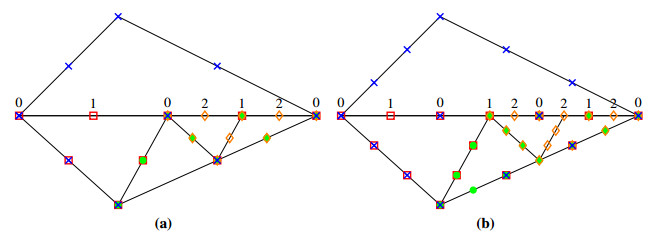
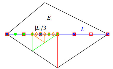
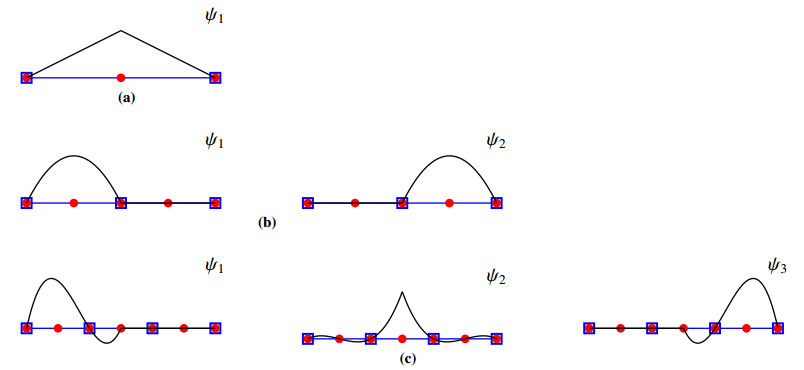
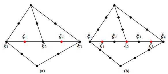
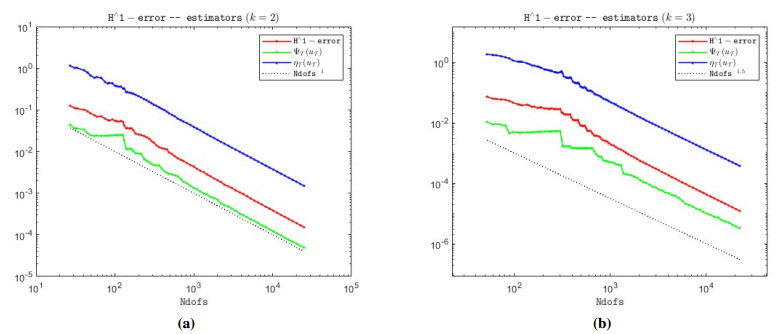
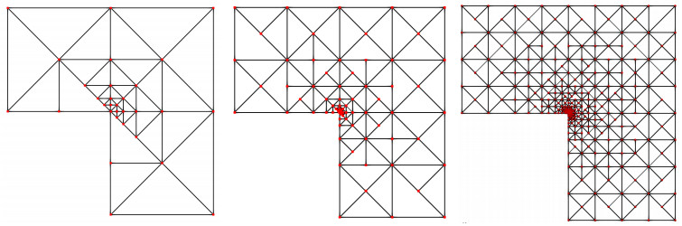
The realization of a standard Adaptive Finite Element Method (AFEM) preserves the mesh conformity by performing a completion step in the refinement loop: In addition to elements marked for refinement due to their contribution to the global error estimator, other elements are refined. In the new perspective opened by the introduction of Virtual Element Methods (VEM), elements with hanging nodes can be viewed as polygons with aligned edges, carrying virtual functions together with standard polynomial functions. The potential advantage is that all activated degrees of freedom are motivated by error reduction, not just by geometric reasons. This point of view is at the basis of the paper [L. Beirão da Veiga et al., "Adaptive VEM: stabilization-free a posteriori error analysis and contraction property", SIAM Journal on Numerical Analysis, vol. 61, 2023], devoted to the convergence analysis of an adaptive VEM generated by the successive newest-vertex bisections of triangular elements without applying completion, in the lowest-order case (polynomial degree $ k = 1 $). The purpose of this paper is to extend these results to the case of VEMs of order $ k\ge2 $ built on triangular meshes. The problem at hand is a variable-coefficient, second-order self-adjoint elliptic equation with Dirichlet boundary conditions; the data of the problem are assumed to be piecewise polynomials of degree $ k-1 $. By extending the concept of global index of a hanging node, under an admissibility assumption of the mesh, we derive a stabilization-free a posteriori error estimator. This is the sum of residual-type terms and certain virtual inconsistency terms (which vanish for $ k = 1 $). We define an adaptive VEM of order $ k $ based on this estimator, and we prove its convergence by establishing a contraction result for a linear combination of (squared) energy norm of the error, (squared) residual estimator, and (squared) virtual inconsistency estimator.
Citation: Claudio Canuto, Davide Fassino. Higher-order adaptive virtual element methods with contraction properties[J]. Mathematics in Engineering, 2023, 5(6): 1-33. doi: 10.3934/mine.2023101
The realization of a standard Adaptive Finite Element Method (AFEM) preserves the mesh conformity by performing a completion step in the refinement loop: In addition to elements marked for refinement due to their contribution to the global error estimator, other elements are refined. In the new perspective opened by the introduction of Virtual Element Methods (VEM), elements with hanging nodes can be viewed as polygons with aligned edges, carrying virtual functions together with standard polynomial functions. The potential advantage is that all activated degrees of freedom are motivated by error reduction, not just by geometric reasons. This point of view is at the basis of the paper [L. Beirão da Veiga et al., "Adaptive VEM: stabilization-free a posteriori error analysis and contraction property", SIAM Journal on Numerical Analysis, vol. 61, 2023], devoted to the convergence analysis of an adaptive VEM generated by the successive newest-vertex bisections of triangular elements without applying completion, in the lowest-order case (polynomial degree $ k = 1 $). The purpose of this paper is to extend these results to the case of VEMs of order $ k\ge2 $ built on triangular meshes. The problem at hand is a variable-coefficient, second-order self-adjoint elliptic equation with Dirichlet boundary conditions; the data of the problem are assumed to be piecewise polynomials of degree $ k-1 $. By extending the concept of global index of a hanging node, under an admissibility assumption of the mesh, we derive a stabilization-free a posteriori error estimator. This is the sum of residual-type terms and certain virtual inconsistency terms (which vanish for $ k = 1 $). We define an adaptive VEM of order $ k $ based on this estimator, and we prove its convergence by establishing a contraction result for a linear combination of (squared) energy norm of the error, (squared) residual estimator, and (squared) virtual inconsistency estimator.

| [1] |
B. Ahmad, A. Alsaedi, F. Brezzi, L. D. Marini, A. Russo, Equivalent projectors for virtual element methods, Comput. Math. Appl., 66 (2013), 376–391. http://dx.doi.org/10.1016/j.camwa.2013.05.015 doi: 10.1016/j.camwa.2013.05.015

|
| [2] |
P. F. Antonietti, F. Dassi, E. Manuzzi, Machine learning based refinement strategies for polyhedra, J. Comput. Phys., 469 (2022), 111531. http://dx.doi.org/10.1016/j.jcp.2022.111531 doi: 10.1016/j.jcp.2022.111531
|
| [3] |
L. Beirão da Veiga, F. Brezzi, A. Cangiani, G. Manzini, L. D. Marini, A. Russo, Basic principles of virtual element methods, Math. Mod. Meth. Appl. Sci., 23 (2013), 199–2014. http://dx.doi.org/10.1142/S0218202512500492 doi: 10.1142/S0218202512500492
|
| [4] |
L. Beirão da Veiga, F. Brezzi, L. D. Marini, A. Russo, The hitchhiker's guide to the virtual element method, Math. Mod. Meth. Appl. Sci., 24 (2014), 1541–1573. http://dx.doi.org/10.1142/S021820251440003X doi: 10.1142/S021820251440003X
|
| [5] |
L. Beirão da Veiga, C. Canuto, R. H. Nochetto, G. Vacca, M. Verani, Adaptive VEM: stabilization-free a posteriori error analysis and contraction property, SIAM J. Numer. Anal., 61 (2023), 457–494. http://dx.doi.org/10.1137/21M1458740 doi: 10.1137/21M1458740
|
| [6] | L. Beirão da Veiga, C. Canuto, R. H. Nochetto, G. Vacca, M. Verani, Adaptive VEM for variable data: convergence and optimality, IMA J. Numer. Anal., 2023. http://dx.doi.org/10.1093/imanum/drad085 |
| [7] |
L. Beirão da Veiga, C. Lovandina, A. Russo, Stability analysis for the virtual element method, Math. Mod. Meth. Appl. Sci., 27 (2017), 2557–2594. http://dx.doi.org/10.1142/S021820251750052X doi: 10.1142/S021820251750052X
|
| [8] |
L. Beirão da Veiga, G. Manzini, Residual a posteriori error estimation for the virtual element method for elliptic problems, ESAIM: M2AN, 49 (2015), 577–599. http://dx.doi.org/10.1051/m2an/2014047 doi: 10.1051/m2an/2014047
|
| [9] |
S. Berrone, A. Borio, A. D'Auria, Refinement strategies for polygonal meshes applied to adaptive VEM discretization, Finite Elem. Anal. Des., 186 (2021), 103502. http://dx.doi.org/10.1016/j.finel.2020.103502 doi: 10.1016/j.finel.2020.103502
|
| [10] |
S. Berrone, A. D'Auria, A new quality preserving polygonal mesh refinement algorithm for polygonal element methods, Finite Elem. Anal. Des., 207 (2022), 103770. http://dx.doi.org/10.1016/j.finel.2022.103770 doi: 10.1016/j.finel.2022.103770
|
| [11] |
P. Binev, W. Dahmen, R. DeVore, Adaptive finite element methods with convergence rates, Numer. Math., 97 (2004), 219–268. http://dx.doi.org/10.1007/s00211-003-0492-7 doi: 10.1007/s00211-003-0492-7
|
| [12] |
A. Cangiani, E. H. Georgoulis, T. Pryer, O. J. Sutton, A posteriori error estimates for the virtual element method, Numer. Math., 137 (2017), 857–893. http://dx.doi.org/10.1007/s00211-017-0891-9 doi: 10.1007/s00211-017-0891-9
|
| [13] | C. Carstensen, M. Feischl, M. Page, D. Praetorius, Axioms of adaptivity, Comput. Math. Appl., 67 (2014), 1195–1253. http://dx.doi.org/10.1016/j.camwa.2013.12.003 |
| [14] |
J. M. Cascon, C. Kreuzer, R. H. Nochetto, K. G. Siebert, Quasi-optimal convergence rate for an adaptive finite element method, SIAM J. Numer. Anal., 46 (2008), 2524–2550. http://dx.doi.org/10.1137/07069047X doi: 10.1137/07069047X
|
| [15] |
W. Dörfler, A convergent adaptive algorithm for Poisson's equation, SIAM J. Numer. Anal., 33 (1996), 1106–1124. http://dx.doi.org/10.1137/0733054 doi: 10.1137/0733054
|
| [16] |
F. D. Gaspoz, P. Morin, Approximation classes for adaptive higher order finite element approximation, Math. Comp., 83 (2014), 2127–2160. http://dx.doi.org/10.1090/s0025-5718-2013-02777-9 doi: 10.1090/s0025-5718-2013-02777-9
|
| [17] |
F. D. Gaspoz, P. Morin, Errata to "Approximation classes for adaptive higher order finite element approximation", Math. Comp., 86 (2017), 1525–1526. http://dx.doi.org/10.1090/mcom/3243 doi: 10.1090/mcom/3243
|
| [18] | R. H. Nochetto, A. Veeser, Primer of adaptive finite element methods, In: S. Bertoluzza, R. H. Nochetto, A. Quarteroni, K. G. Siebert, A. Veeser, Multiscale and adaptivity: modeling, numerics and applications, Lecture Notes in Mathematics, Berlin, Heidelberg: Springer, 2040 (2012), 125–225. http://dx.doi.org/10.1007/978-3-642-24079-9 |

Figures(7) / Tables(1)

Claudio Canuto, Davide Fassino. Higher-order adaptive virtual element methods with contraction properties[J]. Mathematics in Engineering, 2023, 5(6): 1-33. doi: 10.3934/mine.2023101


 DownLoad: