Citation: Boumediene Abdellaoui, Ireneo Peral, Ana Primo. A note on the Fujita exponent in fractional heat equation involving the Hardy potential[J]. Mathematics in Engineering, 2020, 2(4): 639-656. doi: 10.3934/mine.2020029
[1] | Veliappan Vijayaraj, Chokkalingam Ravichandran, Thongchai Botmart, Kottakkaran Sooppy Nisar, Kasthurisamy Jothimani . Existence and data dependence results for neutral fractional order integro-differential equations. AIMS Mathematics, 2023, 8(1): 1055-1071. doi: 10.3934/math.2023052 |
[2] | Mohammed A. Almalahi, Satish K. Panchal, Fahd Jarad, Mohammed S. Abdo, Kamal Shah, Thabet Abdeljawad . Qualitative analysis of a fuzzy Volterra-Fredholm integrodifferential equation with an Atangana-Baleanu fractional derivative. AIMS Mathematics, 2022, 7(9): 15994-16016. doi: 10.3934/math.2022876 |
[3] | Muneerah AL Nuwairan, Ahmed Gamal Ibrahim . The weighted generalized Atangana-Baleanu fractional derivative in banach spaces- definition and applications. AIMS Mathematics, 2024, 9(12): 36293-36335. doi: 10.3934/math.20241722 |
[4] | Ismail Gad Ameen, Dumitru Baleanu, Hussien Shafei Hussien . Efficient method for solving nonlinear weakly singular kernel fractional integro-differential equations. AIMS Mathematics, 2024, 9(6): 15819-15836. doi: 10.3934/math.2024764 |
[5] | Muhammad Farman, Ali Akgül, Kottakkaran Sooppy Nisar, Dilshad Ahmad, Aqeel Ahmad, Sarfaraz Kamangar, C Ahamed Saleel . Epidemiological analysis of fractional order COVID-19 model with Mittag-Leffler kernel. AIMS Mathematics, 2022, 7(1): 756-783. doi: 10.3934/math.2022046 |
[6] | Muhammad Imran Asjad, Waqas Ali Faridi, Adil Jhangeer, Maryam Aleem, Abdullahi Yusuf, Ali S. Alshomrani, Dumitru Baleanu . Nonlinear wave train in an inhomogeneous medium with the fractional theory in a plane self-focusing. AIMS Mathematics, 2022, 7(5): 8290-8313. doi: 10.3934/math.2022462 |
[7] | Iman Ben Othmane, Lamine Nisse, Thabet Abdeljawad . On Cauchy-type problems with weighted R-L fractional derivatives of a function with respect to another function and comparison theorems. AIMS Mathematics, 2024, 9(6): 14106-14129. doi: 10.3934/math.2024686 |
[8] | Kishor D. Kucche, Sagar T. Sutar, Kottakkaran Sooppy Nisar . Analysis of nonlinear implicit fractional differential equations with the Atangana-Baleanu derivative via measure of non-compactness. AIMS Mathematics, 2024, 9(10): 27058-27079. doi: 10.3934/math.20241316 |
[9] | Miguel Vivas-Cortez, Muhammad Uzair Awan, Sehrish Rafique, Muhammad Zakria Javed, Artion Kashuri . Some novel inequalities involving Atangana-Baleanu fractional integral operators and applications. AIMS Mathematics, 2022, 7(7): 12203-12226. doi: 10.3934/math.2022678 |
[10] | Ravi Agarwal, Snezhana Hristova, Donal O'Regan . Integral presentations of the solution of a boundary value problem for impulsive fractional integro-differential equations with Riemann-Liouville derivatives. AIMS Mathematics, 2022, 7(2): 2973-2988. doi: 10.3934/math.2022164 |
Fractional differential equations are thought to be the most effective models for a variety of pertinent events. This makes it possible to investigate the existence, uniqueness, controllability, stability, and other properties of analytical solutions. For example, applying conservation laws to the fractional Black-Scholes equation in Lie symmetry analysis, finding existence solutions for some conformable differential equations, and finding existence solutions for some classical and fractional differential equations on the basis of discrete symmetry analysis, for more details, see [1,2,3,4,5].
Atangana and Baleanu unified and extended the definition of Caputo-Fabrizio [5] by introducing exciting derivatives without singular kernel. Also, the same authors presented the derivative containing Mittag-Leffler function as a nonlocal and nonsingular kernel. Many researchers showed their interest in this definition because it opens many and sober directions and carries Riemann-Liouville and Caputo derivatives [6,7,8,9,10,11,12,13].
A variety of problems in economic theory, control theory, global analysis, fractional analysis, and nonlinear analysis have been treated by fixed point (FP) theory. The FP method contributes greatly to the fractional differential/integral equations, through which it is possible to study the existence and uniqueness of the solution to such equations [14,15,16,17]. Also, this topic has been densely studied and several significant results have been recorded in [18,19,20,21].
The concepts of mixed monotone property (MMP) and a coupled fixed point (CFP) for a contractive mapping Ξ:χ×χ→χ, where χ is a partially ordered metric space (POMS) have been initiated by Bhaskar and Lakshmikantham [22]. To support these ideas, they presented some CFP theorems and determined the existence and uniqueness of the solution to a periodic boundary value problem [23,24,25]. Many authors worked in this direction and obtained some nice results concerned with CFPs in various spaces [26,27,28].
Definition 1.1. [22] Consider a set χ≠∅. A pair (a,b)∈χ×χ is called a CFP of the mapping Ξ:χ×χ→χ if a=Ξ(a,b) and b=Ξ(b,a).
Definition 1.2. [22] Assume that (χ,≤) is a partially ordered set and Ξ:χ×χ→χ is a given mapping. We say that Ξ has a MMP if for any a,b∈χ,
a1,a2∈χ, a1≤a2⇒Ξ(a1,b)≤Ξ(a2,b), |
and
b1,b2∈χ, b1≤b2⇒Ξ(a,b1)≥Ξ(a,b2). |
Theorem 1.1. [22] Let (χ,≤,d) be a complete POMS and Ξ:χ×χ→χ be a continuous mapping having the MMP on χ. Assume that there is a τ∈[0,1) so that
d(Ξ(a,b),Ξ(k,l))≤τ2(d(a,k)+d(b,l)), |
for all a≥k and b≤l. If there are a0,b0∈χ so that a0≤Ξ(a0,b0) and b0≥Ξ(b0,a0), then Ξ has a CFP, that is, there exist a0,b0∈χ such that a=Ξ(a,b) and b=Ξ(b,a).
The same authors proved that Theorem 1.1 is still valid if we replace the hypothesis of continuity with the following: Assume χ has the property below:
(†) if a non-decreasing sequence {am}→a, then am≤a for all m;
(‡) if a non-increasing sequence {bm}→b, then b≤bm for all m.
The following auxiliary results are taken from [29,30], which are used efficiently in the next section.
Let Θ represent a family of non-decreasing functions θ:[0,∞)→[0,∞) so that ∑∞m=1θm(τ)<∞ for all τ>0, where θn is the n-th iterate of θ justifying:
(i) θ(τ)=0⇔τ=0;
(ii) for all τ>0, θ(τ)<τ;
(iii) for all τ>0, lims→τ+θ(s)<τ.
Lemma 1.1. [30] If θ:[0,∞)→[0,∞) is right continuous and non-decreasing, then limm→∞θm(τ)=0 for all τ≥0 iff θ(τ)<τ for all τ>0.
Let ˜L be the set of all functions ˜ℓ:[0,∞)→[0,1) which verify the condition:
limm→∞˜ℓ(τm)=1 implies limm→∞τm=0. |
Recently, Samet et al. [29] reported exciting FP results by presenting the concept of α-θ-contractive mappings.
Definition 1.3. [29] Let χ be a non empty-set, Ξ:χ→χ be a map and α:χ×χ→R be a given function. Then, Ξ is called α-admissible if
α(a,b)≥1⇒α(Ξa,Ξb))≥1, ∀a,b∈χ. |
Definition 1.4. [29] Let (χ,d) be a metric space. Ξ:χ→χ is called an α-θ-contractive mapping, if there exist two functions α:χ×χ→[0,+∞) and θ∈Θ such that
α(a,b)d(Ξ(a,b))≤θ(d(a,b)), |
for all a,b∈χ.
Theorem 1.2. [29] Let (χ,d) be a metric space, Ξ:χ→χ be an α-ψ-contractive mapping justifying the hypotheses below:
(i) Ξ is α-admissible;
(ii) there is a0∈χ so that α(a0,Ξa0)≥1;
(iii) Ξ is continuous.
Then Ξ has a FP.
Moreover, the authors in [29] showed that Theorem 1.2 is also true if we use the following condition instead of the continuity of the mapping Ξ.
● If {am} is a sequence of χ so that α(am,am+1)≥1 for all m and limm→+∞am=a∈χ, then for all m, α(am,a)≥1.
The idea of an α-admissible mapping has spread widely, and the FPs obtained under this idea are not small, for example, see [31,32,33,34].
Furthermore, one of the interesting directions for obtaining FPs is to introduce the idea of Geraghty contractions [30]. The author [30] generalized the Banach contraction principle and obtained some pivotal results in a complete metric space. It is worth noting that a good number of researchers have focused their attention on this idea, for example, see [35,36,37]. In respect of completeness, we state Geraghty's theorem.
Theorem 1.3. [30] Let Ξ:χ→χ be an operator on a complete metric space (χ,d). Then Ξ has a unique FP if Ξ satisfies the following inequality:
d(Ξa,Ξb)≤˜ℓ(d(a,b))d(a,b), for any a,b∈χ, |
where ˜ℓ∈˜L.
We need the following results in the last part.
Definition 1.5. [5] Let σ∈H1(s,t), s<t, and ν∈[0,1). The Atangana–Baleanu fractional derivative in the Caputo sense of σ of order ν is described by
(ABCsDνσ)(ζ)=Q(ν)1−νζ∫sσ′(ϑ)Mν(−ν(ζ−ϑ)ν1−ν)dϑ, |
where Mν is the Mittag-Leffler function given by Mν(r)=∞∑m=0rmΓ(mν+1) and Q(ν) is a normalizing positive function fulfilling Q(0)=Q(1)=1 (see [4]). The related fractional integral is described as
(ABsIνσ)(ζ)=1−νQ(ν)σ(ζ)+νQ(ν)(sIνσ)(ζ), | (1.1) |
where sIν is the left Riemann-Liouville fractional integral defined by
(sIνσ)(ζ)=1Γ(ν)ζ∫s(ζ−ϑ)ν−1σ(ϑ)dϑ. | (1.2) |
Lemma 1.2. [38] For ν∈(0,1), we have
(ABsIνABCDνσ)(ζ)=σ(ζ)−σ(s). |
The outline for this paper is as follows: In Section 1, we presented some known consequences about α-admissible mappings and some useful definitions and theorems that will be used in the sequel. In Section 2, we introduce an ηℓθ-contraction type mapping and obtain some related CFP results in the context of POMSs. Also, we support our theoretical results with some examples. In Section 5, an application to find the existence of a solution for the Atangana-Baleanu coupled fractional differential equation (CFDE) in the Caputo sense is presented.
Let L be the set of all functions ℓ:[0,∞)→[0,1) satisfying the following condition:
limm→∞ℓ(τn)=1 implies limm→∞τn=1. |
We begin this part with the following definitions:
Definition 2.1. Suppose that Ξ:χ×χ→χ and η:χ2×χ2→[0,∞) are two mappings. The mapping Ξ is called η-admissible if
η((a,b),(k,l))≥1⇒η((Ξ(a,b),Ξ(b,a)),(Ξ(k,l),Ξ(l,k)))≥1, ∀a,b,k,l∈χ. |
Definition 2.2. Let (χ,ϖ) be a POMS and Ξ:χ×χ→χ be a given mapping. Ξ is termed as an ηℓθ-coupled contraction mapping if there are two functions η:χ2×χ2→[0,∞) and θ∈Θ so that
η((a,b),(k,l))ϖ(Ξ(a,b),Ξ(k,l))≤ℓ(θ(ϖ(a,k)+ϖ(b,l)2))θ(ϖ(a,k)+ϖ(b,l)2), | (2.1) |
for all a,b,k,l∈χ with a≥k and b≤l, where ℓ∈L.
Remark 2.1. Notice that since ℓ:[0,∞)→[0,1), we have
η((a,b),(k,l))ϖ(Ξ(a,b),Ξ(k,l))≤ℓ(θ(ϖ(a,k)+ϖ(b,l)2))×θ(ϖ(a,k)+ϖ(b,l)2)<θ(ϖ(a,k)+ϖ(b,l)2), for any a,b,k,l∈χ with a≠b≠k≠l. |
Theorem 2.1. Let (χ,≤,ϖ) be a complete POMS and Ξ be an ηℓθ-coupled contraction which has the mixed monotone property so that
(i) Ξ is η-admissible;
(ii) there are a0,b0∈χ so that
η((a0,b0),(Ξ(a0,b0),Ξ(b0,a0)))≥1 and η((b0,a0),(Ξ(b0,a0),Ξ(a0,b0)))≥1; |
(iii) Ξ is continuous.
If there are a0,b0∈χ so that a0≤Ξ(a0,b0) and b0≥Ξ(b0,a0), then Ξ has a CFP.
Proof. Let a0,b0∈χ be such that η((a0,b0),(Ξ(a0,b0),Ξ(b0,a0)))≥1, η((b0,a0),(Ξ(b0,a0),Ξ(a0,b0)))≥1, a0≤Ξ(a0,b0)=a1 (say) and b0≥Ξ(b0,a0)=b1 (say). Consider a2,b2∈χ so that Ξ(a1,b1)=a2 and Ξ(b1,a1)=b2. Similar to this approach, we extract two sequences {am} and {bm} in χ so that
am+1=Ξ(am,bm) and bm+1=Ξ(bm,am), for all m≥0. |
Now, we shall show that
am≤am+1 and bm≥bm+1, for all m≥0. | (2.2) |
By a mathematical induction, we have
(1) At m=0, because a0≤Ξ(a0,b0) and b0≥Ξ(b0,a0) and since Ξ(a0,b0)=a1 and Ξ(b0,a0)=b1, we obtain a0≤a1 and b0≥b1, thus (2.2) holds for m=0.
(2) Suppose that (2.2) holds for some fixed m≥0.
(3) Attempting to prove the validity of (2.2) for any m, by assumption (2) and the mixed monotone property of Ξ, we get
am+2=Ξ(am+1,bm+1)≥Ξ(am,bm+1)≥Ξ(am,bm)=am+1, |
and
bm+2=Ξ(bm+1,am+1)≤Ξ(bm,am+1)≤Ξ(bm,am)=bm+1. |
This implies that
am+2≥am+1 and bm+2≤bm+1. |
Thus, we conclude that (2.2) is valid for all n≥0.
Next, if for some m≥0, (am+1,bm+1)=(am,bm), then am=Ξ(am,bm) and bm=Ξ(bm,am), i.e., Ξ has a CFP. So, let (am+1,bm+1)≠(am,bm) for all m≥0. As Ξ is η-admissible, we get
η((a0,b0),(a1,b1))=η((a0,b0),(Ξ(a0,b0),Ξ(b0,a0)))≥1, |
implies
η((Ξ(a0,b0),Ξ(b0,a0)),(Ξ(a1,b1),Ξ(b1,a1)))=η((a1,b1),(a2,b2))≥1. |
Thus, by induction, one can write
η((am,bm),(am+1,bm+1))≥1 and η((bm,am),(bm+1,am+1))≥1 for all m≥0. | (2.3) |
Using (2.1) and (2.3) and the definition of ℓ, we have
ϖ(am,am+1)=ϖ(Ξ(am−1,bm−1),Ξ(am,bm))≤η((am−1,bm−1),(am,bm))ϖ(Ξ(am−1,bm−1),Ξ(am,bm))≤ℓ(θ(ϖ(am−1,am)+ϖ(bm−1,bm)2))θ(ϖ(am−1,am)+ϖ(bm−1,bm)2)≤θ(ϖ(am−1,am)+ϖ(bm−1,bm)2). | (2.4) |
Analogously, we get
ϖ(bm,bm+1)=ϖ(Ξ(bm−1,am−1),Ξ(bm,am))≤η((bm−1,am−1),(bm,am))ϖ(Ξ(bm−1,am−1),Ξ(bm,am))≤θ(ϖ(bm−1,bm)+ϖ(am−1,am)2). | (2.5) |
Adding (2.4) and (2.5) we have
ϖ(am,am+1)+ϖ(bm,bm+1)2≤θ(ϖ(am−1,am)+ϖ(bm−1,bm)2). |
Continuing in the same way, we get
ϖ(am,am+1)+ϖ(bm,bm+1)2≤θm(ϖ(a0,a1)+ϖ(b0,b1)2), for all m∈N. |
For ϵ>0, there exists m(ϵ)∈N so that
∑m≥m(ϵ)θm(ϖ(a0,a1)+ϖ(b0,b1)2)<ϵ2, |
for some θ∈Θ. Let m,j∈N be so thatj>m>m(ϵ). Then based on the triangle inequality, we obtain
ϖ(am,aj)+ϖ(bm,bj)2≤j−1∑i=mϖ(ai,ai+1)+ϖ(bi,bi+1)2≤j−1∑i=mθi(ϖ(a0,a1)+ϖ(b0,b1)2)≤∑m≥m(ϵ)θm(ϖ(a0,a1)+ϖ(b0,b1)2)<ϵ2, |
this leads to ϖ(am,aj)+ϖ(bm,bj)<ϵ. Because
ϖ(am,aj)≤ϖ(am,aj)+ϖ(bm,bj)<ϵ, |
and
ϖ(bm,bj)≤ϖ(am,aj)+ϖ(bm,bj)<ϵ, |
hence {am} and {bm} are Cauchy sequences in χ. The completeness of χ implies that the sequences {am} and {bm} are convergent in χ, that is, there are a,b∈χ so that
limm→∞am=a and limm→∞bm=b. |
Since Ξ is continuous, am+1=Ξ(am,bm) and bm+1=Ξ(bm,am), we obtain after taking the limit as m→∞ that
a=limm→∞am=limm→∞Ξ(am−1,bm−1)=Ξ(a,b), |
and
b=limm→∞bm=limm→∞Ξ(bm−1,am−1)=Ξ(b,a). |
Therefore, Ξ has a CFP and this ends the proof.
In the above theorem, when omitting the continuity assumption on Ξ, we derive the following theorem.
Theorem 2.2. Let (χ,≤,ϖ) be a complete POMS and Ξ be an ηℓθ-coupled contraction and having the mixed monotone property so that
(a) Ξ is η-admissible;
(b) there are a0,b0∈χ so that
η((a0,b0),(Ξ(a0,b0),Ξ(b0,a0)))≥1 and η((b0,a0),(Ξ(b0,a0),Ξ(a0,b0)))≥1; |
(c) if {am} and {bm} are sequences in χ such that
η((am,bm),(am+1,bm+1))≥1, η((bm,am),(bm+1,am+1))≥1 |
for all m≥0, limm→∞am=a∈χ and limm→∞bm=b∈χ, then
η((am,bm),(a,b))≥1 and η((bm,am),(b,a))≥1. |
If a0,b0∈χ are that a0≤Ξ(a0,b0) and b0≥Ξ(b0,a0), then Ξ has a CFP.
Proof. With the same approach as for the proof of Theorem 2.1, the sequences {am} and {bm} are Cauchy sequences in χ. The completeness of χ implies that there are a,b∈χ so that
limm→∞am=a and limm→∞bm=b. |
According to the assumption (c) and (2.3), one can write
η((am,bm),(a,b))≥1 and η((bm,am),(b,a))≥1, for all m∈N. | (2.6) |
It follows by (2.3), the definition of ℓ and the property of θ(τ)<τ for all τ>0, that
ϖ(Ξ(a,b),a)≤ϖ(Ξ(a,b),Ξ(am,bm))+ϖ(Ξ(am,bm),a)≤η((am,bm),(a,b))ϖ(Ξ(am,bm),Ξ(a,b))+ϖ(am+1,a)≤ℓ(θ(ϖ(am,a)+ϖ(bm,b)2))θ(ϖ(am,a)+ϖ(bm,b)2)+ϖ(am+1,a)≤θ(ϖ(am,a)+ϖ(bm,b)2)+ϖ(am+1,a)<ϖ(am,a)+ϖ(bm,b)2+ϖ(am+1,a). | (2.7) |
Similarly, we find that
ϖ(Ξ(b,a),b)≤ϖ(Ξ(b,a),Ξ(bm,am))+ϖ(Ξ(bm,am),b)≤η((bm,am),(b,a))ϖ(Ξ(bm,am),Ξ(b,a))+ϖ(bm+1,b)≤ℓ(θ(ϖ(bm,b)+ϖ(am,a)2))θ(ϖ(bm,b)+ϖ(am,a)2)+ϖ(bm+1,b)≤θ(ϖ(bm,b)+ϖ(am,a)2)+ϖ(bm+1,b)<ϖ(bm,b)+ϖ(am,a)2+ϖ(bm+1,b). | (2.8) |
As m→∞ in (2.7) and (2.8), we have
ϖ(Ξ(a,b),a)=0 and ϖ(Ξ(b,a),b)=0. |
Hence, a=Ξ(a,b) and b=Ξ(b,a). Thus, Ξ has a CFP and this completes the proof.
In order to show the uniqueness of a CFP, we give the theorem below. If (χ,≤) is a partially ordered set, we define a partial order relation ≤ on the product χ×χ as follows:
(a,b)≤(k,l)⇔a≤k and b≥l, for all (a,b),(k,l)∈χ×χ. |
Theorem 2.3. In addition to the assertions of Theorem 2.1, assume that for each (a,b),(y,z) in χ×χ, there is (k,l)∈χ×χ so that
η((a,b),(k,l))≥1 and η((y,z),(k,l))≥1. |
Suppose also (k,l) is comparable to (a,b) and (y,z). Then Ξ has a unique CFP.
Proof. Theorem 2.1 asserts that the set of CFPs is non-empty. Let (a,b) and (y,z) be CFPs of the mapping Ξ, that is, a=Ξ(a,b), b=Ξ(b,a) and y=Ξ(y,z), z=Ξ(z,y). By hypothesis, there is (k,l)∈χ×χ so that (k,l) is comparable to (a,b) and (y,z). Let (a,b)≤(k,l), k=k0 and l=l0. Choose k1,l1∈χ×χ so that k1=Ξ(k1,l1), l1=Ξ(l1,k1). Thus, we can construct two sequences {km} and {lm} as
km+1=Ξ(km,lm) and lm+1=Ξ(lm,km). |
Since (k,l) is comparable to (a,b), in an easy way we can prove that a≤k1 and b≥l1. Hence, for m≥1, we have a≤km and b≥lm. Because for every (a,b),(y,z)∈χ×χ, there is (k,l)∈χ×χ so that
η((a,b),(k,l))≥1 and η((y,z),(k,l))≥1. | (2.9) |
Because Ξ is η-admissible, then by (2.9), we get
η((a,b),(k,l))≥1 implies η((Ξ(a,b),Ξ(b,a)),(Ξ(k,l),Ξ(l,k)))≥1. |
Since k=k0 and l=l0, we obtain
η((a,b),(k,l))≥1 implies η((Ξ(a,b),Ξ(b,a)),(Ξ(k0,l0),Ξ(l0,k0)))≥1. |
Hence,
η((a,b),(k,l))≥1 implies η((a,b),(k1,l1))≥1. |
So, by induction, we conclude that
η((a,b),(km,lm))≥1, | (2.10) |
for all m∈N. Analogously, one can obtain that η((b,a),(lm,km))≥1. Therefore, the obtained results hold if (a,b)≤(k,l). Based on (2.9) and (2.10), we can write
ϖ(a,km+1)=ϖ(Ξ(a,b),Ξ(km,lm))≤η((a,b),(km,lm))ϖ(Ξ(a,b),Ξ(km,lm))≤ℓ(θ(ϖ(a,km)+ϖ(b,lm)2))θ(ϖ(a,km)+ϖ(b,lm)2)≤θ(ϖ(a,km)+ϖ(b,lm)2). | (2.11) |
Similarly, we get
ϖ(b,lm+1)=ϖ(Ξ(b,a),Ξ(lm,km))≤η((b,a),(lm,km))ϖ(Ξ(b,a),Ξ(lm,km))≤ℓ(θ(ϖ(b,lm)+ϖ(a,km)2))θ(ϖ(b,lm)+ϖ(a,km)2)≤θ(ϖ(b,lm)+ϖ(a,km)2). | (2.12) |
Adding (2.11) and (2.12), we have
ϖ(a,km+1)+ϖ(b,lm+1)2≤θ(ϖ(b,lm)+ϖ(a,km)2). |
Thus,
ϖ(a,km+1)+ϖ(b,lm+1)2≤θm(ϖ(b,l1)+ϖ(a,k1)2), | (2.13) |
for each n≥1. As m→∞ in (2.13) and by Lemma 1.1, we have
limm→∞(ϖ(a,km+1)+ϖ(b,lm+1))=0, |
which yields that
limm→∞ϖ(a,km+1)=limm→∞ϖ(b,lm+1)=0. | (2.14) |
Similarly, one obtains
limm→∞ϖ(y,km+1)=limm→∞ϖ(z,lm+1)=0. | (2.15) |
It follows from (2.14) and (2.15), we find that a=y and b=z. This proves that the CFP is unique.
Examples below support the theoretical results.
Example 2.1. (Linear case) Let ϖ:χ×χ→R be a usual metric on χ=[0,1]. Define the mappings Ξ:χ×χ→χ and η:χ2×χ2→[0,∞) by Ξ(a,b)=(a−b)32 and
η((a,b),(k,l))={32,if a≥b, k≥l,0otherwise, |
for all a,b,k,l∈χ, respectively. Consider
ℓ(θ(ϖ(a,k)+ϖ(b,l)2))θ(ϖ(a,k)+ϖ(b,l)2)−η((a,b),(k,l))ϖ(Ξ(a,b),Ξ(k,l))=ℓ(θ(ϖ(a,k)+ϖ(b,l)2))θ(ϖ(a,k)+ϖ(b,l)2)−32ϖ(Ξ(a,b),Ξ(k,l))=(1|a−k|4+|b−l|4)(|a−k|4+|b−l|4)−32|Ξ(a,b)−Ξ(k,l)|=1−32|132(a−b)−132(k−l)|=1−364|(a−b)−(k−l)|≥0, |
which implies that
η((a,b),(k,l))ϖ(Ξ(a,b),Ξ(k,l))≤ℓ(θ(ϖ(a,k)+ϖ(b,l)2))θ(ϖ(a,k)+ϖ(b,l)2). |
Therefore, (2.1) is fulfilled with ℓ(τ)=1τ and θ(τ)=τ2, for all τ>0. Also, all the hypotheses of Theorem 2.1 are satisfied and (0,0) is the unique CFP of Ξ.
Example 2.2. (Nonlinear case) Let ϖ:χ×χ→R be the usual metric on χ=[0,1]. Define the mappings Ξ:χ×χ→χ and η:χ2×χ2→[0,∞) by Ξ(a,b)=132(ln(1+a)−ln(1+b)) and
η((a,b),(k,l))={43,if a≥b, k≥l,0otherwise, |
for all a,b,k,l∈χ, respectively. Then, we have
ℓ(θ(ϖ(a,k)+ϖ(b,l)2))θ(ϖ(a,k)+ϖ(b,l)2)−η((a,b),(k,l))ϖ(Ξ(a,b),Ξ(k,l))=ℓ(θ(ϖ(a,k)+ϖ(b,l)2))θ(ϖ(a,k)+ϖ(b,l)2)−43ϖ(Ξ(a,b),Ξ(k,l))=(1θ(ϖ(a,k)+ϖ(b,l)2))θ(ϖ(a,k)+ϖ(b,l)2)−43|Ξ(a,b)−Ξ(k,l)|=1−43×32|(ln(1+a)−ln(1+b))−(ln(1+k)−ln(1+l))|=1−124|(ln(1+a1+k)+ln(1+l1+b))|≥1−124(ln(1+|a−k|)+ln(1+|l−b|))≥0. |
Note that we used the property ln(1+a1+k)≤ln(1+(a−k)). Hence,
ℓ(θ(ϖ(a,k)+ϖ(b,l)2))θ(ϖ(a,k)+ϖ(b,l)2)≥η((a,b),(k,l))ϖ(Ξ(a,b),Ξ(k,l)). |
Therefore, (2.1) holds with ℓ(τ)=1τ and θ(τ)=τ2, for all τ>0. Furthermore, all the hypotheses of Theorem 2.1 are fulfilled and (0,0) is the unique CFP of Ξ.
In this section, we apply Theorem 2.2 to discuss the existence solution for the following Atangana–Baleanu fractional differential equation in the Caputo sense:
{(ABC0Dνσ)(ζ)=φ(ζ,σ(ζ),ρ(ζ)),ζ∈I=[0,1],(ABC0Dνρ)(ζ)=φ(ζ,ρ(ζ),σ(ζ)),0≤ν≤1,σ(0)=σ0 and ρ(0)=ρ0, | (3.1) |
where Dν is the Atangana-Baleanu derivative in the Caputo sense of order ν and φ:I×χ×χ→χ is a continuous function with φ(0,σ(0),ρ(0))=0.
Let ϖ:χ×χ→[0,∞) be a function defined by
ϖ(σ,ρ)=‖σ−ρ‖∞=supζ∈I|σ(ζ)−ρ(ζ)|, |
where χ=C(I,R) represents the set of continuous functions. Define a partial order ≤ on χ by
(a,b)≤(k,l)⇔a≤k and b≥l, for all a,b,k,l∈χ. |
It is clear that (χ,≤,ϖ) is a complete POMS.
Now, to discuss the existence solution to the problem (3.1), we describe our hypotheses in the following theorem:
Theorem 3.1. Assume that:
(h1) there is a continuous function φ:I×χ×χ→χ so that
|φ(ℵ,σ(ℵ),ρ(ℵ))−φ(ℵ,σ∗(ℵ),ρ∗(ℵ))|≤Q(ν)Γ(ν)(1−ν)Γ(ν)+1ℓ(θ(|σ(ℵ)−σ∗(ℵ)|+|ρ(ℵ)−ρ∗(ℵ)|2))×θ(|σ(ℵ)−σ∗(ℵ)|+|ρ(ℵ)−ρ∗(ℵ)|2), |
for ℵ∈I, ℓ∈L, θ∈Θ and σ,ρ,σ∗,ρ∗∈χ. Moreover, there exists ℑ:C2(I)×C2(I)→C(I) such that ℑ((σ(ℵ),ρ(ℵ)),(σ∗(ℵ),ρ∗(ℵ)))≥0 and ℑ((ρ(ℵ),σ(ℵ)),(ρ∗(ℵ),σ∗(ℵ)))≥0, for each σ,ρ,σ∗,ρ∗∈C(I) and ℵ∈I;
(h2) there exist σ1,ρ1∈C(I) with ℑ((σ1(ℵ),ρ1(ℵ)),(Ξ(σ1(ℵ),ρ1(ℵ)),Ξ(ρ1(ℵ),σ1(ℵ))))≥0 and ℑ((ρ1(ℵ),σ1(ℵ)),(Ξ(ρ1(ℵ),σ1(ℵ)),Ξ(σ1(ℵ),ρ1(ℵ))))≥0, for ℵ∈I, where Ξ:C(I)×C(I)→C(I) is defined by
Ξ(ρ,σ)(ℵ)=σ0+AB0Iνφ(ℵ,σ(ℵ),ρ(ℵ)); |
(h3) for σ,ρ,σ∗,ρ∗∈C(I) and ℵ∈I, ℑ((σ(ℵ),ρ(ℵ)),(σ∗(ℵ), ρ∗(ℵ)))≥0 and ℑ((ρ(ℵ),σ(ℵ)), (ρ∗(ℵ),σ∗(ℵ)))≥0 implies
ℑ((Ξ(σ(ℵ),ρ(ℵ)),Ξ(ρ(ℵ),σ(ℵ))),(Ξ(σ∗(ℵ),ρ∗(ℵ)),Ξ(ρ∗(ℵ),σ∗(ℵ))))≥0 |
and
ℑ((Ξ(ρ(ℵ),σ(ℵ)),Ξ(σ(ℵ),ρ(ℵ))),(Ξ(ρ∗(ℵ),σ∗(ℵ)),Ξ(σ∗(ℵ),ρ∗(ℵ))))≥0; |
(h4) if {σm},{ρm}⊆C(I), limm→∞σm=σ, limm→∞ρm=ρ in C(I), ℑ((σm,ρm),(σm+1,ρm+1)) ≥0 and ℑ((ρm,σm), (ρm+1,σm+1))≥0, then ℑ((σm,ρm) ,(σ,ρ))≥0 and ℑ((ρm,σm) ,(ρ,σ))≥0, for all m∈N.
Then there is at least one solution for the problem (3.1).
Proof. Effecting the Atangana-Baleanu integral to both sides of (3.1) and applying Lemma 1.2, we have
σ(ℵ)=σ0+AB0Iνφ(ℵ,σ(ℵ),ρ(ℵ)), |
and
ρ(ℵ)=ρ0+AB0Iνφ(ℵ,ρ(ℵ),σ(ℵ)). |
Now, we shall prove that the mapping Ξ:C(I)×C(I)→C(I) has a CFP. From (1.1) and (1.2) and (h1), we get
|Ξ(ρ,σ)(ℵ)−Ξ(ρ∗,σ∗)(ℵ)|=|AB0Iν[φ(ℵ,σ(ℵ),ρ(ℵ))−φ(ℵ,σ∗(ℵ),ρ∗(ℵ))]|=|1−νQ(ν)[φ(ℵ,σ(ℵ),ρ(ℵ))−φ(ℵ,σ∗(ℵ),ρ∗(ℵ))]+νQ(ν) 0Iν[φ(ℵ,σ(ℵ),ρ(ℵ))−φ(ℵ,σ∗(ℵ),ρ∗(ℵ))]|≤1−νQ(ν)|φ(ℵ,σ(ℵ),ρ(ℵ))−φ(ℵ,σ∗(ℵ),ρ∗(ℵ))|+νQ(ν) 0Iν|φ(ℵ,σ(ℵ),ρ(ℵ))−φ(ℵ,σ∗(ℵ),ρ∗(ℵ))|≤1−νQ(ν)×Q(ν)Γ(ν)(1−ν)Γ(ν)+1ℓ(θ(|σ(ℵ)−σ∗(ℵ)|+|ρ(ℵ)−ρ∗(ℵ)|2))×θ(|σ(ℵ)−σ∗(ℵ)|+|ρ(ℵ)−ρ∗(ℵ)|2)+νQ(ν)×Q(ν)Γ(ν)(1−ν)Γ(ν)+1 0Iν(1)ℓ(θ(|σ(ℵ)−σ∗(ℵ)|+|ρ(ℵ)−ρ∗(ℵ)|2))×θ(|σ(ℵ)−σ∗(ℵ)|+|ρ(ℵ)−ρ∗(ℵ)|2)={Q(ν)Γ(ν)(1−ν)Γ(ν)+1ℓ(θ(|σ(ℵ)−σ∗(ℵ)|+|ρ(ℵ)−ρ∗(ℵ)|2))×θ(|σ(ℵ)−σ∗(ℵ)|+|ρ(ℵ)−ρ∗(ℵ)|2)}(1−νQ(ν)+νQ(ν)νΓ(ν))≤{Q(ν)Γ(ν)(1−ν)Γ(ν)+1ℓ(θ(supℵ∈I|σ(ℵ)−σ∗(ℵ)|+supℵ∈I|ρ(ℵ)−ρ∗(ℵ)|2))×θ(supℵ∈I|σ(ℵ)−σ∗(ℵ)|+supℵ∈I|ρ(ℵ)−ρ∗(ℵ)|2)}(1−νQ(ν)+νQ(ν)νΓ(ν))=(Q(ν)Γ(ν)(1−ν)Γ(ν)+1ℓ(θ(ϖ(σ,σ∗)+ϖ(ρ,ρ∗)2))θ(ϖ(σ,σ∗)+ϖ(ρ,ρ∗)2))×(1−νQ(ν)+1Q(ν)Γ(ν))=ℓ(θ(ϖ(σ,σ∗)+ϖ(ρ,ρ∗)2))θ(ϖ(σ,σ∗)+ϖ(ρ,ρ∗)2). |
Hence, for σ,ρ∈C(I), ℵ∈I, with ℑ((σ(ℵ),ρ(ℵ)),(σ∗(ℵ),ρ∗(ℵ)))≥0 and ℑ((ρ(ℵ),σ(ℵ)),(ρ∗(ℵ),σ∗(ℵ)))≥0, we get
ϖ(Ξ(ρ,σ)(ℵ),Ξ(ρ∗,σ∗))≤ℓ(θ(ϖ(σ,σ∗)+ϖ(ρ,ρ∗)2))θ(ϖ(σ,σ∗)+ϖ(ρ,ρ∗)2). |
Define η:C2(I)×C2(I)→[0,∞) by
η((σ(ℵ),ρ(ℵ)),(σ∗(ℵ),ρ∗(ℵ)))={1,if ℑ((σ(ℵ),ρ(ℵ)),(σ∗(ℵ),ρ∗(ℵ)))≥0,0,otherwise. |
So
η((σ(ℵ),ρ(ℵ)),(σ∗(ℵ),ρ∗(ℵ)))ϖ(Ξ(ρ,σ)(ℵ),Ξ(ρ∗,σ∗))≤ℓ(θ(ϖ(σ,σ∗)+ϖ(ρ,ρ∗)2))θ(ϖ(σ,σ∗)+ϖ(ρ,ρ∗)2). |
Then, Ξ is an ηℓθ-coupled contraction mapping. Now, for each ρ,σ,ρ∗,σ∗∈C(I) and ℵ∈I, we have
η((σ(ℵ),ρ(ℵ)),(σ∗(ℵ),ρ∗(ℵ)))≥1, |
due to definition of ℑ and η. So, hypothesis (h3) gives
{η((Ξ(σ(ℵ),ρ(ℵ)),Ξ(ρ(ℵ),σ(ℵ))),(Ξ(σ∗(ℵ),ρ∗(ℵ)),Ξ(ρ∗(ℵ),σ∗(ℵ))))≥1,η((Ξ(ρ(ℵ),σ(ℵ)),Ξ(σ(ℵ),ρ(ℵ))),(Ξ(ρ∗(ℵ),σ∗(ℵ)),Ξ(σ∗(ℵ),ρ∗(ℵ))))≥1, |
for ρ,σ,ρ∗,σ∗∈C(I). Therefore, Ξ is η-admissible. From (h2), there are σ0,ρ0∈C(I) with η((σ0(ℵ),ρ0(ℵ)),Ξ(σ0(ℵ),ρ0(ℵ)))≥1 and η((ρ0(ℵ),σ0(ℵ)),Ξ(ρ0(ℵ),σ0(ℵ)))≥1. Using (h4) and Theorem 2.2, we conclude that there is (ˆσ,ˆρ)∈C(I) with ˆσ=Ξ(ˆσ,ˆρ) and ˆρ=Ξ(ˆρ,ˆσ), that is, Ξ has a CFP, which is a solution of the system (3.1).
Many physical phenomena can be described by nonlinear differential equations (both ODEs and PDEs), so the study of numerical and analytical methods used in solving nonlinear differential equations are an interesting topic for analyzing scientific engineering problems. From this perspective, some coupled fixed point results for the class of ηℓθ-contractions in POMSs are obtained. These results are reinforced by their applications in a study of the existence of a solution for a CFDE with the Mittag-Leffler kernel. In the future, our findings may be applied to differential equations of an arbitrary fractional order, linear and nonlinear fractional integro-differential systems, Hadamard fractional derivatives, Caputo-Fabrizio's kernel, and so on.
This work was supported in part by the Basque Government under Grant IT1555-22.
The authors declare that they have no competing interests.
[1] |
Abdellaoui B, Peral I, Primo A (2009) Influence of the Hardy potential in a semilinear heat equation. P Roy Soc Edinb A 139: 897–926. doi: 10.1017/S0308210508000152
![]() |
[2] |
Abdellaoui B, Medina M, Peral I, et al. (2016) Optimal results for the fractional heat equation involving the Hardy potential. Nonlinear Anal 140: 166–207. doi: 10.1016/j.na.2016.03.013
![]() |
[3] |
Baras P, Goldstein JA (1984) The heat equation with a singular potential. T Am Math Soc 284: 121–139. doi: 10.1090/S0002-9947-1984-0742415-3
![]() |
[4] | Barrios B, Medina M, Peral I (2014) Some remarks on the solvability of non-local elliptic problems with the Hardy potential. Commun Contemp Math 16: 1–29. |
[5] | Beckner W (1995) Pitt's inequality and the uncertainty principle. P Am Math Soc 123: 1897–1905. |
[6] | Blumenthal RM, Getoor RK (1969) Some theorems on stable processes. T Am Math Soc 95: 263– 273. |
[7] | Caffarelli L, Figalli A (2013) Regularity of solutions to the parabolic fractional obstacle problem. J Reine Angew Math 680: 191–233. |
[8] |
Di Nezza E, Palatucci G, Valdinoci E (2012) Hitchhiker's guide to the fractional Sobolev spaces. Bull Sci Math 136: 521–573. doi: 10.1016/j.bulsci.2011.12.004
![]() |
[9] | Frank R, Lieb EH, Seiringer R (2008) Hardy-Lieb-Thirring inequalities for fractional Schrödinger operators. J Am Math Soc 20: 925–950. |
[10] | Fujita H (1966) On the blowing up of solutions of the Cauchy problem for ut = ∆u + u1+α. J Fac Sci Univ Tokyo Sect I 13: 109–124. |
[11] |
Guedda M, Kirane M (2001) Criticality for some evolution equations. Diff Equat 37: 540–550. doi: 10.1023/A:1019283624558
![]() |
[12] |
Herbst IW (1977) Spectral theory of the operator (p2 + m2)1/2 - Ze2/r. Commun Math Phys 53: 285–294. doi: 10.1007/BF01609852
![]() |
[13] |
Kobayashi K, Sino T, Tanaka H (1977) On the growing-up problem for semilinear heat equations. J Math Soc JPN 29: 407–424. doi: 10.2969/jmsj/02930407
![]() |
[14] | Landkof N (1972) Foundations of Modern Potential Theory, Springer-Verlag. |
[15] |
Leonori T, Peral I, Primo A, et al. (2015) Basic estimates for solutions of a class of nonlocal elliptic and parabolic equations. Discrete Cont Dyn A 35: 6031–6068. doi: 10.3934/dcds.2015.35.6031
![]() |
[16] | Mitidieri E, Pohozhaev SI (2014) A Priori Estimates and Blow-up of Solutions to Nonlinear Partial Differential Equations and Inequalities, Proceedings of the Steklov Institute of Mathematics. |
[17] | Peral I, Soria F (2021) Elliptic and Parabolic Equations involving the Hardy-Leray Potential. |
[18] | Polya G (1923) On the zeros of an integral function represented by Fourier's integral. Messenger Math 52: 185–188. |
[19] | Quittner P, Souplet P (2007) Superlinear Parabolic Problems Blow-up, Global Existence and Steady States, Birkhauser, Basel, Switzerland. |
[20] | Riesz M (1938) Intégrales de Riemann-Liouville et potenciels. Acta Sci Math Szeged 9: 1–42. |
[21] |
Silvestre L (2012) On the differentiability of the solution to an equation with drift and fractional diffusion. Indiana U Math J 61: 557–584. doi: 10.1512/iumj.2012.61.4568
![]() |
[22] | Sugitani S (1975) On nonexistence of global solutions for some nonlinear integral equations. Osaka J Math 12: 45–51. |
[23] | Stein EM, Weiss G (1958) Fractional integrals on n-dimensional Euclidean space. J Math Mech 7: 503–514. |
[24] |
Weissler F (1981) Existence and nonexistence of global solutions for a semilinear heat equation. Israel Mat 38: 29–40. doi: 10.1007/BF02761845
![]() |
[25] | Yafaev D (1999) Sharp constants in the Hardy-Rellich inequalities. J Funct Anal 168: 12–144. |
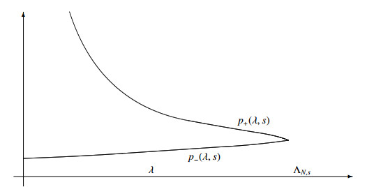
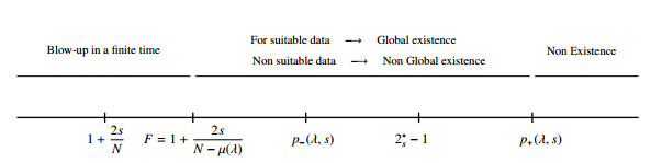