Marine microfossils: Tiny archives of ocean changes through deep time

Jasenka Sremac; Marija Bošnjak; Karmen Fio Firi; Ana Šimičević; Šimun Aščić; Jasenka Sremac; Marija Bošnjak; Karmen Fio Firi; Ana Šimičević; Šimun Aščić

doi:10.3934/microbiol.2024030

AIMS Microbiology

2024, Volume 10, Issue 3: 644-673. doi: 10.3934/microbiol.2024030

Previous Article Next Article

Review

Marine microfossils: Tiny archives of ocean changes through deep time

1.
University of Zagreb, Faculty of Science, Department of Geology, Horvatovac 102B, 10000 Zagreb, Croatia
2.
Croatian Natural History Museum, Demetrova 1, 10000 Zagreb, Croatia
3.
Franka Lisice 4, 23000 Zadar, Croatia

Received: 05 April 2024 Revised: 08 July 2024 Accepted: 25 July 2024 Published: 08 August 2024

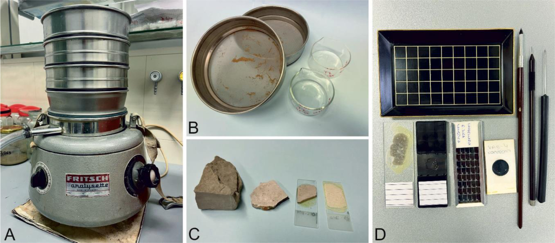
Microorganisms have inhabited the oceans since the dawn of Earth. Some of them have organic walls and some produce mineral tests that are usually composed of carbonate minerals or silica. They can therefore be preserved with original parts during sedimentary deposition or fossilized through permineralization or carbonization processes. The most common marine fossil groups studied by micropaleontologists are cyanobacteria, coccolithophores, dinoflagellates, diatoms, silicoflagellates, radiolarians, foraminifers, red and green algae, ostracods, and pteropods. Dormant or reproductive cysts can also be used for determinations of the fossil microbiota. Microfossils can be studied in petrographic slides prepared from rocks or separated from loosely consolidated rocks by disaggregation or dissolution and wet sieving. Their presence is sometimes recognized by biomarkers. Transmitted light microscopy and reflected light stereomicroscopy are necessary for micropaleontological studies whereas scanning electronic microscopy (SEM) aids research on the tiniest fossils and reveals fine skeletal details. Microorganisms have influenced the oxygenation of water and the atmosphere, as well as Earth's carbon cycle and have contributed to the formation of sedimentary rocks. By studying microfossils, paleontologists depict the age of the rock and identify depositional environments. Such studies help us recognize periods of stress in Earth's history and understand their influence on living organisms. Biogenic rocks, made of microfossils, can be used as raw materials, such as fossil fuels, building stone, or additives for the food industry, agricultural, or cosmetic purposes.
- microbiota,
- fossilization,
- biostratigraphy,
- paleoenvironment,
- raw materials
Citation: Jasenka Sremac, Marija Bošnjak, Karmen Fio Firi, Ana Šimičević, Šimun Aščić. Marine microfossils: Tiny archives of ocean changes through deep time[J]. AIMS Microbiology, 2024, 10(3): 644-673. doi: 10.3934/microbiol.2024030

Related Papers:

Abstract

Microorganisms have inhabited the oceans since the dawn of Earth. Some of them have organic walls and some produce mineral tests that are usually composed of carbonate minerals or silica. They can therefore be preserved with original parts during sedimentary deposition or fossilized through permineralization or carbonization processes. The most common marine fossil groups studied by micropaleontologists are cyanobacteria, coccolithophores, dinoflagellates, diatoms, silicoflagellates, radiolarians, foraminifers, red and green algae, ostracods, and pteropods. Dormant or reproductive cysts can also be used for determinations of the fossil microbiota. Microfossils can be studied in petrographic slides prepared from rocks or separated from loosely consolidated rocks by disaggregation or dissolution and wet sieving. Their presence is sometimes recognized by biomarkers. Transmitted light microscopy and reflected light stereomicroscopy are necessary for micropaleontological studies whereas scanning electronic microscopy (SEM) aids research on the tiniest fossils and reveals fine skeletal details. Microorganisms have influenced the oxygenation of water and the atmosphere, as well as Earth's carbon cycle and have contributed to the formation of sedimentary rocks. By studying microfossils, paleontologists depict the age of the rock and identify depositional environments. Such studies help us recognize periods of stress in Earth's history and understand their influence on living organisms. Biogenic rocks, made of microfossils, can be used as raw materials, such as fossil fuels, building stone, or additives for the food industry, agricultural, or cosmetic purposes.

Acknowledgments

Results of our research were partly obtained through the Croatian Science Foundation Project “Sedimentary paleobasins, water corridors and biota migrations” (IP-2019-04-7042), led by Marijan Kovačić (University of Zagreb, Faculty of Science).
We are grateful to Kristina Pikelj (University of Zagreb, Faculty of Science) for providing diatom and silicoflagellate remains, and Duje Kukoč (Croatian Geological Survey) for radiolarian images.
Authors would like to thank the reviewers and editors for their constructive and helpful comments, which have significantly improved the quality of this paper.

Conflict of interest

The authors declare no conflict of interest.

Author contributions

Conceptualization, J.S., M.B.; methodology, K.F.F., M.B., Š.A., A.Š.; validation, J.S. and M.B.; resources, J.S., M.B., K.F.F., A.Š, Š.A.; writing—original draft preparation, J.S., M.B., K.F.F.; writing review and editing, J.S., K.F.F., M.B.; visualization, J.S., M.B., K.F.F., A.Š, Š.A.; supervision, J.S., K.F.F. and M.B.
All authors have read and agreed to the published version of the manuscript.

References

[1]	Moore TC, Echols RJ (1979) Micropaleontology, Paleontology. Encyclopedia of Earth Science. Berlin, Heidelberg: Springer 470-475. https://doi.org/10.1007/3-540-31078-9_85
[2]	Siesser WG (1981) Christian Gottfried Ehrenberg: Founder of micropaleontology. Centaurus 25: 166-188. https://doi.org/10.1111/j.1600-0498.1981.tb00643.x
[3]	Grote M (2022) Microbes before microbiology: Christian Gottfried Ehrenberg and Berlin's infusoria. Endeavour 46: 100815. https://doi.org/10.1016/j.endeavour.2022.100815
[4]	Slipper IJ (2005) Micropaleontological techniques. Encyclopedia of Geology. New York: Academic Press 470-475. https://doi.org/10.1016/B0-12-369396-9/00105-2
[5]	Green OR (2001) A Manual of Practical Laboratory and Field Techniques in Palaeobiology. Berlin, Heidelberg: Springer. https://doi.org/10.1007/978-94-017-0581-3
[6]	Pekčec M Middle Miocene fossil communities of Kladje area, Sv. Nedelja (2019).
[7]	Pezelj Đ, Sremac J, Bermanec V (2016) Shallow-water benthic foraminiferal assemblages and their response to the palaeoenvironmental changes–example from the Middle Miocene of Medvednica Mt. (Croatia, Central Paratethys). Geol Carpath 67: 329-345. https://doi.org/10.1515/geoca-2016-0021
[8]	Bošnjak M, Sremac J, Vrsaljko D, et al. (2017) Miocene “Pteropod event” in the SW part of the Central Paratethys (Medvednica Mt., northern Croatia). Geol Carpath 68: 329-349. https://doi.org/10.1515/geoca-2017-0023
[9]	Butterfield NJ (2014) Early evolution of the Eukaryota. Palaeontol 58: 5-17. https://doi.org/10.1111/pala.12139
[10]	Knoll AH (2014) Paleobiological perspectives on early Eukaryotic evolution. Cold Spring Harbor Perspect Biol 6: a016121. https://doi.org/10.1101/cshperspect.a016121
[11]	Mahendrarajah TA, Moody ERR, Schrempf D, et al. (2023) ATP synthase evolution on a cross-braced dated tree of life. Nat Commun 14: 7456. https://doi.org/10.1038/s41467-023-42924-w
[12]	Riding R (2011) The nature of stromatolites: 3,500 million years of history and a century of research, Advances in Stromatolite Geobiology. Lecture Notes in Earth Sciences. Berlin, Heidelberg: Springer 29-74. https://doi.org/10.1007/978-3-642-10415-2_3
[13]	Holland.Volcanic gases, black smokers, and the great oxidation event. Geochim Cosmochim Acta (2002) 66: 3811-3826. https://doi.org/10.1016/S0016-7037(02)00950-X
[14]	Shields-Zhou G, Och L (2011) The case for a Neoproterozoic oxygenation event: Geochemical evidence and biological consequences. GSA Today 21: 4-11. http://dx.doi.org/10.1130/GSATG102A.1
[15]	Sremac J, Fio K Geological lolocality and trails in the National park Mljet (2010). Available from: https://www.croris.hr/crosbi/publikacija/prilog-skup/572631
[16]	Palinkaš LA, Sremac J (1987) Barite-bearing stromatolites at the Permian–Triassic boundary in Gorski Kotar (Croatia, Yugoslavia). Mem Soc Geol It 40: 259-264.
[17]	Foster WJ, Heindel K, Richoz S, et al. (2020) Suppressed competitive exclusion enabled the proliferation of Permian/Triassic boundary microbialites. Depos Rec 6: 62-74. https://doi.org/10.1002/dep2.97
[18]	Zhang XY, Wang WQ, Yuan DX, et al. (2020) Stromatolite-dominated microbialites at the Permian–Triassic boundary of the Xikou section on South Qinling Block, China. Palaeoworld 29: 126-136. https://doi.org/10.1016/j.palwor.2019.05.009
[19]	Bacteria: Fossil Record. Available from: https://ucmp.berkeley.edu/bacteria/bacteriafr.html
[20]	Šimičević A, Sremac J Cyclic sedimentation in marginal marine shelf environment at the Middle/Upper Permian boundary in central part of the Velebit Mt., Croatia (2014). Available from: http://geol.pmf.hr/~jsremac/radovi/znanstveni/2014_srbija_velebit.pdf
[21]	Majstorović Bušić A Stratigraphic, petroleum geological and paleoecological features of the Sarmatian deposits in the western part of the Sava depression [dissertation] (2019). Available from: https://urn.nsk.hr/urn:nbn:hr:217:679703
[22]	Monteiro FM, Bach LT, Brownlee C, et al. (2016) Why marine phytoplankton calcify. Sci Adv 2: e1501822. https://doi.org/10.1126/sciadv.1501822
[23]	Balch WM, Bowler BC, Drapeau DT, et al. (2019) Coccolithophore distributions of the North and South Atlantic Ocean. Deep Sea Research Part I 151: 103066. https://doi.org/10.1016/j.dsr.2019.06.012
[24]	Choudari PP, Patil SM, Mohan R (2020) Use of coccolith based proxies for palaeoceanographic reconstructions. Curr Sci 119: 307-315. https://doi.org/10.18520/cs/v119/i2/307-315
[25]	MIRACLECalcareous Nannofossils. Available from: https://www.ucl.ac.uk/GeolSci/micropal/calcnanno.html
[26]	Bernoulli D, Jenkyns HC (2023) Thomas Henry Huxley, a stone tablet, coccoliths, and deep-sea sediments in the high Alps. Int J Earth Sci 112: 1661-1669. https://doi.org/10.1007/s00531-023-02330-5
[27]	Lohmann H (1902) Die Coccolithporidae. Arch Protistenk 1: 89-165.
[28]	Holligan PM (1992) Do marine phytoplankton influence global climate. Primary Productivity and Biogeochemical Cycles in the Sea. New Zork: Plenum Press 487-501.
[29]	Giradeau J, Beaufirt L (2007) Coccolithophores: From extant populations to fossil assemblages. Developments in Marine Geology. Amsterdam: Elsevier. https://doi.org/10.1016/S1572-5480(07)01015-9
[30]	Kinkel H, Baumann KH, Cepek M (2000) Coccolithophores in the equatorial Atlantic Ocean: Response to seasonal and Late Quaternary surface water variability. Mar Micropaleontol 39: 87-112. https://doi.org/10.1016/S0377-8398(00)00016-5
[31]	Earth ObservatoryCoccolithophores. Available from: https://earthobservatory.nasa.gov/features/Coccolithophores/coccolith_3.php
[32]	Riding JB, Fensome RA, Soyer-Gobillard MO, et al. (2023) A review of the Dinoflagellates and their evolution from fossils to modern. J Mar Sci Eng 11: 1. https://doi.org/10.3390/jmse11010001
[33]	Volkman J, Kearney P, Jeffrey S (1990) A new source of 4-methyl sterols and 5α(H)-stanols in sediments: Prymnesiophyte microalgae of the genus Pavlova. Org Geochem 15: 489-497. https://doi.org/10.1016/0146-6380(90)90094-G
[34]	Fensome RA, Taylor FJR, Norris G, et al. (1993) A classification of living and fossil dinoflagellates. Micropaleonotology. Hanover: Sheridan Press.
[35]	de Verteuil L, Norris G (1996) Miocene dinoflagellate stratigraphy and systematics of Maryland and Virginia. Micropaleontology 42. https://doi.org/10.2307/1485926
[36]	Bakrač K, Koch G, Sremac J (2012) Middle and Late Miocene palynological biozonation of the south-western part of Central Paratethys (Croatia). Geol Croat 65: 207-222. https://doi.org/10.4154/GC.2012.12
[37]	Jiménez-Moreno G, Head MJ, Harzhauser M (2006) Early and Middle Miocene dinoflagellate cyst stratigraphy of the central Paratethys, central Europe. J Micropalaeontol 25: 113-139. https://doi.org/10.1144/jm.25.2.113
[38]	Sremac J, Bošnjak M, Velić J, et al. (2022) Nearshore pelagic influence at the SW margin of the Paratethys Sea–examples from the Miocene of Croatia. Geosciences 12: 120. https://doi.org/10.3390/geosciences12030120
[39]	Ślivińska KK (2019) Early Oligocene dinocysts as a tool for palaeoenvironment reconstruction and stratigraphical framework–a case study from the North Sea well. J Micropalaeontol 38: 143-176. https://doi.org/10.5194/jm-38-143-2019
[40]	Nezhad AAJ, Ghasemi-Nejad, Ghasemi-Nejad E (2016) Paleocene–Oligocene dinoflagellate cysts from the Siah Anticline, Zagros Basin, Southwest Iran. Geol USP Sér Cient 16: 25-35. https://doi.org/10.11606/issn.2316-9095.v16i2p25-35
[41]	MIRACLEAcritarchs and Chitinozoa. Available from: https://www.ucl.ac.uk/GeolSci/micropal/acritarch.html
[42]	Diatoms. Available from: https://diatoms.org/
[43]	Pikelj K, Hernitz-Kučenjak M, Aščić Š, et al. (2015) Surface sediment around the Jabuka Islet and the Jabuka Shoal: Evidence of Miocene tectonics in the Central Adriatic Sea. Mar Geol 359: 120-133. http://dx.doi.org/10.1016/j.margeo.2014.11.003
[44]	Li Z, Zhang Y, Li W, et al. (2023) Common environmental stress responses in a model marine diatom. New Phytol 240: 272-284. https://doi.org/10.1111/nph.19147
[45]	Pierella Karlusich JJ, Ibarbalz FM, Bowler C (2020) Exploration of marine phytoplankton: from their historical appreciation to the omics era. J Plankton Res 42: 595-612. https://doi.org/10.1093/plankt/fbaa049
[46]	Bryłka K, Alverson AJ, Pickering RA, et al. (2023) Uncertainties surrounding the oldest fossil record of diatoms. Sci Rep 13: 8047. https://doi.org/10.1038/s41598-023-35078-8
[47]	Diatoms: Fossil Record. Available from: https://ucmp.berkeley.edu/chromista/diatoms/diatomfr.html
[48]	Flower RJ, Williams DM (2023) Diatomites: Their formation, distribution and uses. Reference Module in Earth Systems and Environmental Sciences. Amsterdam: Elsevier. https://doi.org/10.1016/B978-0-323-99931-1.00080-5
[49]	Łach M, Pławecka K, Marczyk J, et al. (2023) Use of diatomite from Polish fields in sustainable development as a sorbent for petroleum substances. J Clean Prod 389: 136100. https://doi.org/10.1016/j.jclepro.2023.136100
[50]	Rothwell RG (2016) Sedimentary rocks: Deep ocean pelagic oozes. Earth Systems and Environmental Sciences. Amsterdam: Elsevier. https://doi.org/10.1016/B978-0-12-409548-9.10493-2
[51]	Biard T (2022) Diversity and ecology of Radiolaria in modern oceans. Environ Microbiol 24: 2179-2200. https://doi.org/10.1111/1462-2920.16004
[52]	Vukovski M, Kukoč D, Grgasović T, et al. (2023) Evolution of eastern passive margin of Adria recorded in shallow- to deep-water successions of the transition zone between the Alps and the Dinarides (Ivanščica Mt., NW Croatia). Facies 69: 18. https://doi.org/10.1007/s10347-023-00674-7
[53]	Pikelj K Composition and origin of seabed sediments of the eastern part of the Adriatic Sea–in Croatian) (2010). Available from: https://www.croris.hr/crosbi/publikacija/ocjenski-rad/360366
[54]	Valde-Nowak P, Kerneder-Gubała K (2019) Mapping the radiolarite outcrops as potential source of raw material in the Stone Age: Characterisation of Polish part of the Pieniny Klippen Belt. Anthropol et Præhist 128: 157-174.
[55]	Taylor EL, Taylor TN, Krings M (2008) Paleobotany: The Biology and Evolution of Fossil Plants. New York: Academic Press 1-1252.
[56]	McCartney K (2013) A review of past and recent research on Cretaceous silicoflagellates. Phytotaxa 127: 190-200. https://doi.org/10.11646/phytotaxa.127.1.18
[57]	Perch-Nielsen K (1985) Silicoflagellates. Plankton Stratigraphy. Cambridge: Cambridge University Press 811-846.
[58]	Bajraktarević Z (1983) Middle Miocene (Badenian and Lower Sarmatian) nannofossils in Northern Croatia. Paleont Jugosl 30: 5-23.
[59]	Bajraktarević Z (1984) The application of microforaminiferal association and nannofossils for biostratigraphic classification of the Middle Miocene of north Croatia. Acta Geol : 1-34.
[60]	Galović I, Bajraktarević Z (2006) Sarmatian biostratigraphy of the Mountain Medvednica at Zagreb based on siliceous microfossils (North Croatia, Central Paratethys). Geol Carpath 57: 199-210.
[61]	BritannicaForaminiferan. Available from: https://www.britannica.com/science/foraminiferan
[62]	Sremac J, Huić F, Bošnjak M, et al. (2024) The composition of acervulinid-red algal macroids from the Paleogene of Croatia and their distribution in the wider Mediterranean region. Recent Research on Sedimentology, Stratigraphy, Paleontology, Geochemistry, Volcanology, Tectonics and Petroleum Geology. Berlin, Heidelberg: Springer 59-62. https://doi.org/10.1007/978-3-031-48758-3_14
[63]	Cook T, Abbott L Travels in Geology: The pyramids of Giza: Wonders of an ancient world (2018). Available from: https://www.earthmagazine.org/article/travels-geology-pyramids-giza-wonders-ancient-world/
[64]	Fio K Biotic and abiotic proxies of stress events across the Permian–Triassic Boundary in the area of the Velebit Mt (2010). Available from: https://www.croris.hr/crosbi/publikacija/ocjenski-rad/362486
[65]	Kolar-Jurkovšek T, Jurkovšek B, Aljinović D (2011) Conodont biostratigraphy and lithostratigraphy across the Permian–Triassic boundary at the Luka section in western Slovenia. Riv Ital Paleontol S 117: 115-133.
[66]	Krainer K, Vachard D (2011) The Lower Triassic Werfen Formation of the Karawanken Mountains (Southern Austria) and its disaster survivor microfossils, with emphasis on Postcladella n. gen. (Foraminifera, Miliolata, Cornuspirida). R Micropaleontol 54: 59-85. https://doi.org/10.1016/j.revmic.2008.11.001
[67]	Murray JW (1991) Ecology and paleoecology of benthic foraminifera. Longmann Scientific and Technical, Harlow : 1-397.
[68]	Kochansky-Devidé, V (1973) Trogkofel Beds in Croatia. Geol vjesn 26: 41-51. Available from: https://geoloski-vjesnik.hgi-cgs.hr/wp-content/uploads/2022/07/1973_Kochansky-Devide_441.pdf
[69]	Palatinuš I, Gobo K, Fio Firi K, et al. (2024) Lower Permian Košna conglomerates of the Velebit Mt. (Croatia): Modal composition, provenance and depositional environment. Geol Croat 77: 1-14. https://doi.org/10.4154/gc.2024.02
[70]	International Commission on Stratigraphy. Available from: https://stratigraphy.org/chart
[71]	Fio Firi K, Sremac J, Vlahović I (2016) The first evidence of Permian–Triassic shallow-marine transitional deposits in northern Croatia: Samoborsko Gorje Hills. Swiss J Geosci 109: 401-413. https://doi.org/10.1007/s00015-016-0233-4
[72]	Van der Zwaan GJ, Jorssen FJ, de Stigter HC (1990) The depth dependency of planktonic/benthic foraminiferal ratios: Constraints and applications. Mar Geol 95: 1-16. https://doi.org/10.1016/0025-3227(90)90016-D
[73]	Van der Zwaan GJ, Dujinstee IAP, den Dulk M, et al. (1999) Benthic foraminiferes: proxies or problems? A review of palaeoecological concepts. Earth Sci Rev 46: 213-236. https://doi.org/10.1016/S0012-8252(99)00011-2
[74]	Hohenegger J (2005) Estimation of environmental palaeogradient values based on presence/absence data: A case study using benthic foraminifera for palaeodepth estimation. Palaeogeogr Palaeoclimatol Palaeoecol 217: 115-130. https://doi.org/10.1016/j.palaeo.2004.11.020
[75]	Báldi K, Hohenegger J (2008) Palaeoecology of benthic foraminifera of the Baden–Sooss section (Badenian, Middle Miocene, Vienna Basin, Austria). Geol Carpath 59: 411-424.
[76]	Hammer Ø, Harper DAT, Ryan PD (2001) Past: Paleontological statistics software package for education and data analysis. Palaeontol Electron 4: 1-9. http://palaeo-electronica.org/2001_1/past/issue1_01.htm
[77]	Pezelj Đ, Drobnjak L (2019) Foraminifera-based estimation of water depth in epicontinental seas: Badenian deposits from Glavnica Gornja (Medvednica Mt., Croatia), Central Paratethys. Geol Croat 72: 93-100. https://doi.org/10.4154/gc.2019.08
[78]	McCorkle DC, Corliss BH, Farnham CA (1997) Vertical distributions and stable isotopic compositions of live (stained) benthic foraminifera from the North Carolina and California continental margins. Deep Sea Res Part I 44: 983-1024. https://doi.org/10.1016/S0967-0637(97)00004-6
[79]	Bemis BE, Spero HJ, Bijma J, et al. (1998) Reevaluation of the oxygen isotopic composition of planktonic foraminifera: experimental results and revised paleotemperature equations. Paleoceanography 13: 150-160. https://doi.org/10.1029/98PA00070
[80]	Báldi K (2006) Paleoceanography and climate of the Badenian (Middle Miocene, 16.4–13.0 Ma) in the Central Paratethys based on foraminifera and stable isotope (δ¹⁸O and δ¹³C) evidence. Int J Earth Sci 95: 119-142. https://doi.org/10.1007/s00531-005-0019-9
[81]	Kováčová P, Emmanuel L, Hudáčková N, et al. (2009) Central Paratethys paleoenvironment during the Badenian (Middle Miocene): Evidence from foraminifera and stable isotope (δ¹³C and δ¹⁸O) study in the Vienna Basin (Slovakia). Int J Earth Sci 98: 1109-1127. https://doi.org/10.1007/s00531-008-0307-2
[82]	Hohenegger J, Ćorić S, Wagreich M (2014) Timing of the Middle Miocene Badenian stage of the Central Paratethys. Geol Carpatha 65: 55-66. https://doi.org/10.2478/geoca-2014-0004
[83]	Scheiner F, Holcová K, Milovský R, et al. (2018) Temperature and isotopic composition of seawater in the epicontinental sea (Central Paratethys) during the Middle Miocene Climatic Transition based on Mg/Ca, δ¹⁸O and δ¹³C from foraminiferal tests. Palaeogeogr Palaeoclimatol Palaeoecol 495: 60-71. https://doi.org/10.1016/j.palaeo.2017.12.027
[84]	Repac M Diagenesis impact on paleotemperatures calculated from stable isotopes of foraminifera tests: example from Miocene in Croatia (2017).
[85]	Bengtson S, Sallstedt T, Belivanova V, et al. (2017) Three-dimensional preservation of cellular and subcellular structures suggests 1.6 billion-year-old crown-group red algae. PLoS Biol 15: e2000735. https://doi.org/10.1371/journal.pbio.2000735
[86]	Sissini MN, Koerich G, de Barros-Barreto MB, et al. (2022) Diversity, distribution, and environmental drivers of coralline red algae: The major reef builders in the Southwestern Atlantic. Coral Reefs 41: 711-725. https://doi.org/10.1007/s00338-021-02171-1
[87]	The Marine Life Information NetworkMaerl beds. Available from: https://www.marlin.ac.uk/habitats/detail/255/maerl_beds
[88]	Rhodophyta: Fossil Record. Available from: https://ucmp.berkeley.edu/protista/reds/rhodofr.html
[89]	Sremac J, Huić F, Bošnjak M, et al. Morphometric characteristics and origin of Paleogene macroids from beach gravels in Stanići (vicinity of Omiš, Southern Croatia) (2020). Available from: http://geol.pmf.hr/~jsremac/radovi/znanstveni/2020_Morphometric%20characteristics%20and%20origin%20of%20Palaeogene.pdf
[90]	Herak M, Kochansky-Devidé V (1960) Gymnocodiacean calcareous algae in the Permian of Yugoslavia. Geol vjesn 13: 185-195.
[91]	Sremac J (1991) Zone Neoschwagerina craticulifera in the Middle Velebit Mt. (Croatia, Yugoslavia). Geologija 34: 7-55. https://doi.org/10.5474/geologija.1991.001
[92]	Hughes GW (2017) Exceptionally well-preserved Permocalculus cf. tenellus (Pia) (Gymnocodiaceae) from Upper Permian Khuff Formation limestones, Saudi Arabia. JM 36: 166-173. https://doi.org/10.1144/jmpaleo2016-005
[93]	Basso D, Vrsaljko D, Grgasović T (2008) The coralline flora of a Miocene maërl: The Croatian “Litavac”. Geol Croat 61: 333-340. https://doi.org/10.4154/gc.2008.25
[94]	Sremac J, Bošnjak Makovec M, Vrsaljko D, et al. (2016) Reefs and bioaccumulation in the Miocene deposits of the North Croatian Basin–Amazing diversity yet to be described. Rud-geol-naf zb 31: 19-29. https://doi.org/10.17794/rgn.2016.1.2
[95]	Sremac J, Tripalo K, Repac M, et al. (2018) Middle Miocene drowned ramp in the vicinity of Marija Bistrica (Northern Croatia). Rud-geol-naf zb 33: 23-43. https://doi.org/10.17794/rgn.2018.4.3
[96]	Fio Firi K, Maričić A (2020) Usage of the natural stones in the city of Zagreb (Croatia) and its geotouristical aspect. Geoheritage . https://doi.org/10.1007/s12371-020-00488-x
[97]	Maričić A, Briševac Z, Hrženjak P, et al. (2023) Natural building stone in the construction and renovation of the Zagreb cathedral. Rud-geol-naft zb 38: 29-42. https://doi.org/10.17794/rgn.2023.3.3
[98]	Naselli-Flores L, Barone R (2009) Green Algae. Encyclopedia of Inland Waters. New York: Academic Press 166-173. https://doi.org/10.1016/B978-012370626-3.00134-4
[99]	Berger S (2006) Photo-Atlas of living Dasycladales. Carnets Geol . https://hal.archives-ouvertes.fr/hal-00167300
[100]	Parkovi DinaridaAbout Dinarides. Available from: https://parksdinarides.org/en/about-dinarides/
[101]	Granier B, Leithers A (2017) Draconisella mortoni sp. nov., a Mizzia like Dasycladalean alga from the Lower Cretaceous of Oman. Palaeontol Electron . https://doi.org/10.26879/743
[102]	Granier B, Sander NJ (2013) The XXIst century (the 100^th anniversary) edition of the “new studies on Triassic Siphoneae verticillatae” by Julius von Pia. Carnets Geol . https://doi.org/10.4267/2042/48735
[103]	Granier B, Deloffre R (1993) Reappraisal of the fossil Dasycladalean algae. II: Jurassic and Cretaceous Dasycladalean algae. Rev Paléobiol 12: 19-65.
[104]	Granier B, Grgasović T (2000) Les Algues Dasycladales du Permien et du Trias Nouvelle tentative d'inventaire bibliographique, géographique et stratigraphique. Geol Croat 53: 1-197. Available from: http://www.geologia-croatica.hr/index.php/GC/article/view/GC.2000.01
[105]	Pierrot-Bults AC, Peijnenburg KTCA (2015) Pteropods. Encyclopedia of Marine Geosciences. Berlin, Heidelberg: Springer 680-687. http://dx.doi.org/10.1007/978-94-007-6644-0_88-1
[106]	Janssen AW, Peijnenburg KTCA (2017) An overview of the fossil record of Pteropoda (Mollusca, Gastropoda, Heterobranchia). Cainozoic Res 17: 3-10.
[107]	Cahuzac B, Janssen AW (2010) Eocene to Miocene holoplanktonic Mollusca (Gastropoda) of the Aquitaine Basin, southwest France. Scr Geol 141: 1-193.
[108]	Derežić I, Bošnjak M, Sremac J Biostatistic analyses of newly found pteropods (Mollusca, Gastropoda) in the Middle Miocene (Badenian) deposits from the southeastern Medvednica Mt. (Northern Croatia) (2018). Available from: https://www.bib.irb.hr:8443/969368
[109]	Janssen AW, Zorn I (1993) Revision of Middle Miocene holoplanktonic gastropods from Poland, published by the late Wilhelm Krach. Scr Geol 2: 155-236.
[110]	Zorn I (1991) A systematic account of Tertiary pteropoda (Gastropoda, Euthecosomata) from Austria. Con Tert Quatern Geol 28: 95-139.
[111]	Zorn I (1995) Planktonische Gastropoden (Euthecosomata und Heteropoda) in der Sammlung Mayer-Eymar im naturhistorischen museum in Basel. Eclogae Geol Helv 88: 743-759.
[112]	Zorn I (1999) Planktonic gastropods (pteropods) from the Miocene of the Carpathian Foredeep and the Ždánice Unit in Moravia (Czech Republic). Abh Geol Bundes 56: 723-738.
[113]	Bohn-Havas M, Lantos M, Selmeczi I (2004) Biostratigraphic studies and correlation of Tertiary planktonic gastropods (pteropods) from Hungary. Acta Palaeont Rom 4: 37-43.
[114]	Jovanović G, Bošnjak M, Sremac J, et al. (2024) The Middle Miocene (Badenian) holoplanktonic mollusks (Euthecosomata–Pteropoda) from Serbia, Central Paratetys. Geol An Balk Poluostrva . https://doi.org/10.2298/GABP240229008J
[115]	Bednaršek N, Harvey CJ, Kaplan IC, et al. (2016) Pteropods on the edge: Cumulative effects of ocean acidification, warming, and deoxygenation. Progr Oceanogr 145: 1-24. https://doi.org/10.1016/j.pocean.2016.04.002
[116]	Yousef E (2018) Distribution and taxonomy of shallow marine ostracods from the western coast of the Red Sea, Egypt. Open J Mar Sci 8: 51-75. https://doi.org/10.4236/ojms.2018.81004
[117]	Hajek-Tadesse V, Prtoljan B (2011) Badenian Ostracoda from the Pokupsko area (Banovina, Croatia). Geol Carpath 62: 447-461. https://doi.org/10.2478/v10096-011-0032-9
[118]	Bartha IR, Botka D, Csoma V, et al. (2022) From marginal outcrops to basin interior: A new perspective on the sedimentary evolution of the eastern Pannonian Basin. Int J Earth Sci 111: 335-357. https://doi.org/10.1007/s00531-021-02117-6
[119]	Boomer I, Horne DJ, Slipper IJ (2003) The use of ostracods in palaeoenvironmental studies, or what can you do with an ostracod shell?. Paleont Soc Papers 9: 153-180. https://doi.org/10.1017/S1089332600002199
[120]	Hajek-Tadesse V, Belak M, Sremac J, et al. (2009) Early Miocene ostracods from the Sadovi section (Mt. Požeška gora, Croatia). Geol Carpath 60: 251-262. https://doi.org/10.2478/v10096-009-0017-0
[121]	Janz H, Vennemann TW (2005) Isotopic composition and trace element ratios of Miocene marine and brackish ostracods from north Alpine Foreland deposits as indicators for palaeoclimate. Palaeogeogr Palaeoclimatol Palaeoecol 225: 216-247. https://doi.org/10.1016/j.palaeo.2005.06.012
[122]	Chai S, Hua H, Ren J, et al. (2021) Vase-shaped microfossils from the late Ediacaran Dengying Formation of Ningqiang, South China: Taxonomy, preservation and biological affinity. Precambrian Res 352: 105968. https://doi.org/10.1016/j.precamres.2020.105968
[123]	Tingle KE, Porter SM, Raven MR, et al. (2023) Organic preservation of vase-shaped microfossils from the late Tonian Chuar Group, Grand Canyon, Arizona, USA. Geobiology 21: 290-309. https://doi.org/10.1111/gbi.12544
[124]	Morais L, Freitas BT, Fairchild TR, et al. (2021) Diverse vase-shaped microfossils within a Cryogenian glacial setting in the Urucum Formation (Brazil). Precambrian Res 367: 106470. https://doi.org/10.1016/j.precamres.2021.106470
[125]	Butler A (2015) Fossil Focus: The place of small shelly fossils in the Cambrian explosion, and the origin of Animals. Palaeontol Online 5: 1-14. Available from: http://www.palaeontologyonline.com/articles/2015/fossil-focus-place-small-shelly-fossils-cambrian-explosion-origin-animals/
[126]	Eig K The Cambrian explosion, Part 3: Small shellies and small skeletons (2023). Available from: https://karsteneig.no/2023/04/the-cambrian-explosion-part-3-small-shellies-and-small-skeletons/
[127]	Butterfield NJ, Harvey THP (2012) Small carbonaceous fossils (SCFs): A new measure of early Paleozoic paleobiology. Geology 40: 71-74. https://doi.org/10.1130/G32580.1
[128]	MIRACLE: Conodonts. Available from: https://www.ucl.ac.uk/GeolSci/micropal/conodont.html
[129]	Kozur HW, Ramovš A, Wang CY, et al. (1994) The importance of Hindeodus parvus (Conodonta) for the definition of the Permian–Triassic boundary and evaluation of the proposed sections for a global stratotype section and point (GSSP) for the base of the Triassic. Geologija 37: 173-213. https://doi.org/10.5474/geologija.1995.007
[130]	Zhen YY What are conodonts. Available from: https://australian.museum/learn/australia-over-time/fossils/what-are-conodonts/

Reader Comments

Your name:*

Email:*
© 2024 the Author(s), licensee AIMS Press. This is an open access article distributed under the terms of the Creative Commons Attribution License (http://creativecommons.org/licenses/by/4.0)