Increased risk of diabetic ketoacidosis in an Urban, United States, safety-net emergency department in the COVID-19 era

Elizabeth Burner; Lucy Liu; Sophie Terp; Sanjay Arora; Chun Nok Lam; Michael Menchine; Daniel A Dworkis; Sarah Axeen; Elizabeth Burner; Lucy Liu; Sophie Terp; Sanjay Arora; Chun Nok Lam; Michael Menchine; Daniel A Dworkis; Sarah Axeen

doi:10.3934/medsci.2023004

AIMS Medical Science

2023, Volume 10, Issue 1: 37-45. doi: 10.3934/medsci.2023004

Previous Article Next Article

Research article Topical Sections

Increased risk of diabetic ketoacidosis in an Urban, United States, safety-net emergency department in the COVID-19 era

1.
Department of Emergency Medicine, Keck School of Medicine of the University of Southern California, 1200 N State St, Los Angeles, CA 90033, USA
2.
Schaeffer Center for Health Policy and Economics, University of Southern California, Los Angeles, CA 90089, USA
3.
Department of Population and Public Health Sciences, Keck School of Medicine of the University of Southern California, Los Angeles, CA 90033, USA

Received: 19 September 2022 Revised: 24 January 2023 Accepted: 12 February 2023 Published: 24 February 2023

Aims
The incidence of diabetic ketoacidosis (DKA) increased during the COVID-19 pandemic but estimates from low-resource settings are limited. We examined the odds of DKA among emergency department (ED) visits in the Los Angeles County Department of Health Services (DHS) (1) during the COVID-19 pandemic compared to the pre-COVID era, (2) without active COVID infections, and (3) stratified by effect modifiers to identify impacted sub-groups.

Methods
We estimated the odds of DKA from 400,187 ED visits pre-COVID era (March 2019–Feb 2020) and 320,920 ED visits during the COVID era (March 2020–Feb 2021). Our base model estimated the odds of DKA based on the COVID era. Additional specifications stratified by effect modifiers, controlled for confounders, and limited to visits without confirmed COVID-19 disease.

Results
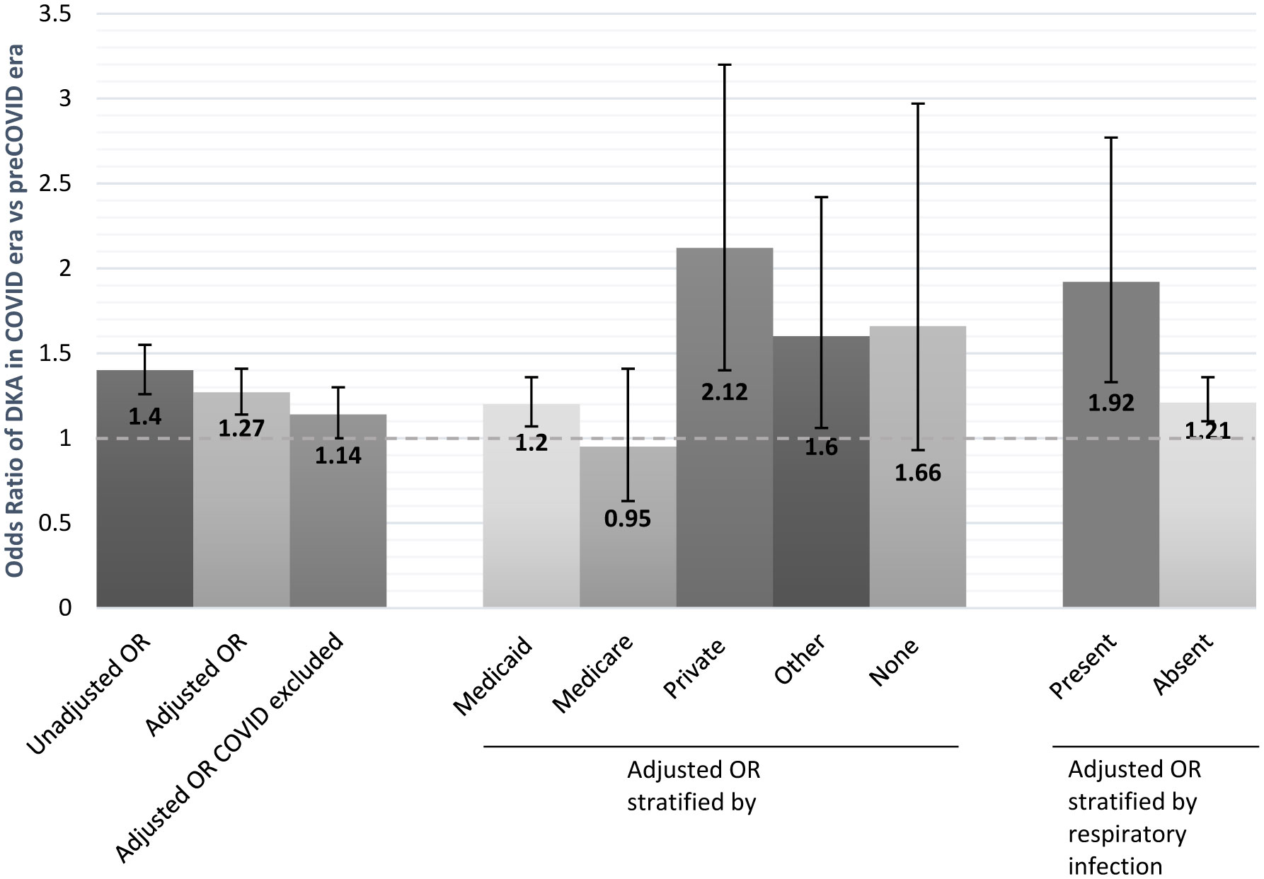
After adjusting for triage acuity and interaction terms for upper respiratory infections and payor, the odds of DKA during the COVID era were 27% higher compared to the pre-COVID era (95%CI 14–41%, p < 0.001). In stratified analyses, visits with private payors had a 112% increased odds and visits with Medicaid had a 20% increased odds of DKA during the COVID era (95%CI 7–36%, p = 0.003).

Conclusions
We identified increased odds of DKA during the COVID pandemic, robust to a variety of specifications. We found differential effects by the payor; with increased odds during COVID for privately-insured patients.
- DKA,
- emergency department,
- COVID-19,
- pandemic,
- insurance,
- access to care
Citation: Elizabeth Burner, Lucy Liu, Sophie Terp, Sanjay Arora, Chun Nok Lam, Michael Menchine, Daniel A Dworkis, Sarah Axeen. Increased risk of diabetic ketoacidosis in an Urban, United States, safety-net emergency department in the COVID-19 era[J]. AIMS Medical Science, 2023, 10(1): 37-45. doi: 10.3934/medsci.2023004

Related Papers:

Abstract

Aims

The incidence of diabetic ketoacidosis (DKA) increased during the COVID-19 pandemic but estimates from low-resource settings are limited. We examined the odds of DKA among emergency department (ED) visits in the Los Angeles County Department of Health Services (DHS) (1) during the COVID-19 pandemic compared to the pre-COVID era, (2) without active COVID infections, and (3) stratified by effect modifiers to identify impacted sub-groups.

Methods

We estimated the odds of DKA from 400,187 ED visits pre-COVID era (March 2019–Feb 2020) and 320,920 ED visits during the COVID era (March 2020–Feb 2021). Our base model estimated the odds of DKA based on the COVID era. Additional specifications stratified by effect modifiers, controlled for confounders, and limited to visits without confirmed COVID-19 disease.

Results

After adjusting for triage acuity and interaction terms for upper respiratory infections and payor, the odds of DKA during the COVID era were 27% higher compared to the pre-COVID era (95%CI 14–41%, p < 0.001). In stratified analyses, visits with private payors had a 112% increased odds and visits with Medicaid had a 20% increased odds of DKA during the COVID era (95%CI 7–36%, p = 0.003).

Conclusions

We identified increased odds of DKA during the COVID pandemic, robust to a variety of specifications. We found differential effects by the payor; with increased odds during COVID for privately-insured patients.

Funding

Dr. Burner's time for this project was partially supported by a grant from the NIDDK K23DK106538.

Conflict of interest

The authors confirm that there are no conflicts of interest in this article's content.

References

[1]	Vellanki P, Umpierrez GE (2021) Diabetic ketoacidosis risk during the COVID-19 pandemic. Lancet Diabetes Endocrinol 9: 643-644. https://doi.org/10.1016/S2213-8587(21)00241-2
[2]	Misra S, Barron E, Vamos E, et al. (2021) Temporal trends in emergency admissions for diabetic ketoacidosis in people with diabetes in England before and during the COVID-19 pandemic: A population-based study. Lancet Diabetes Endocrinol 9: 671-680. https://doi.org/10.1016/S2213-8587(21)00208-4
[3]	Goldman N, Fink D, Cai J, et al. (2020) High prevalence of COVID-19-associated diabetic ketoacidosis in UK secondary care. Diabetes Res Clin Pract 166: 108291. https://doi.org/10.1016/j.diabres.2020.108291
[4]	de Sa-Ferreira CO, da Costa CHM, Guimaraes JCW, et al. (2022) Diabetic ketoacidosis and COVID-19: what have we learned so far?. Am J Physiol Endocrinol Metab 322: E44-E53. https://doi.org/10.1152/ajpendo.00244.2021
[5]	Chao LC, Vidmar AP, Georgia S (2021) Spike in diabetic ketoacidosis rates in pediatric type 2 diabetes during the COVID-19 pandemic. Diabetes Care 44: 1451-1453. https://doi.org/10.2337/dc20-2733
[6]	Hardin EM, Keller DR, Kennedy TP, et al. (2022) An unanticipated worsening of glycemic control following a mild COVID-19 infection. Cureus 14: e26295. https://doi.org/10.7759/cureus.26295
[7]	Lam CN, Axeen S, Terp S, et al. (2021) Who stayed home under safer-at-home? Impacts of COVID-19 on volume and patient-mix at an emergency department. West J Emerg Med 22: 234-243. https://doi.org/10.5811/westjem.2020.12.49234
[8]	Ebekozien O, Agarwal S, Noor N, et al. (2021) Inequities in diabetic ketoacidosis among patients with type 1 diabetes and COVID-19: data from 52 US clinical centers. J Clin Endocrinol Metab 106: e1755-e1762. https://doi.org/10.1210/clinem/dgaa920
[9]	Tilden DR, Datye KA, Moore DJ, et al. (2021) The rapid transition to telemedicine and its effect on access to care for patients with type 1 diabetes during the COVID-19 pandemic. Diabetes Care 44: 1447-1450. https://doi.org/10.2337/dc20-2712
[10]	Patel SY, McCoy RG, Barnett ML, et al. (2021) Diabetes care and glycemic control during the COVID-19 pandemic in the United States. JAMA Intern Med 181: 1412-1414. https://doi.org/10.1001/jamainternmed.2021.3047
[11]	Fisher L, Polonsky W, Asuni A, et al. (2020) The early impact of the COVID-19 pandemic on adults with type 1 or type 2 diabetes: A national cohort study. J Diabetes Complications 34: 107748. https://doi.org/10.1016/j.jdiacomp.2020.107748
[12]	Boddu SK, Aurangabadkar G, Kuchay MS (2020) New onset diabetes, type 1 diabetes and COVID-19. Diabetes Metab Syndr 14: 2211-2217. https://doi.org/10.1016/j.dsx.2020.11.012
[13]	Zhong VW, Juhaeri J, Mayer-Davis EJ (2018) Trends in hospital admission for diabetic ketoacidosis in adults with type 1 and type 2 diabetes in England, 1998–2013: A retrospective cohort study. Diabetes Care 41: 1870-1877. https://doi.org/10.2337/dc17-1583
[14]	Wu CT, Lidsky PV, Xiao Y, et al. (2021) SARS-CoV-2 infects human pancreatic β cells and elicits β cell impairment. Cell Metab 33: 1565-1576.e5. https://doi.org/10.1016/j.cmet.2021.05.013
[15]	Metwally AA, Mehta P, Johnson BS, et al. (2021) COVID-19-induced new-onset diabetes: trends and technologies. Diabetes 70: 2733-2744. https://doi.org/10.2337/dbi21-0029
[16]	Kamrath C, Monkemoller K, Biester T, et al. (2020) Ketoacidosis in children and adolescents with newly diagnosed type 1 diabetes during the COVID-19 pandemic in Germany. JAMA 324: 801-804. https://doi.org/10.1001/jama.2020.13445
[17]	Calamera JC, Giovenco P, Brugo S, et al. (1987) Adenosine 5 triphosphate (ATP) content and acrosin activity in polyzoospermic subjects. Andrologia 19: 460-463. https://doi.org/10.1111/j.1439-0272.1987.tb02328.x
[18]	Chambers MA, Mecham C, Arreola EV, et al. (2022) Increase in the number of pediatric new-onset diabetes and diabetic ketoacidosis cases during the COVID-19 pandemic. Endocr Pract 28: 479-485. https://doi.org/10.1016/j.eprac.2022.02.005

Reader Comments

Your name:*

Email:*
© 2023 the Author(s), licensee AIMS Press. This is an open access article distributed under the terms of the Creative Commons Attribution License (http://creativecommons.org/licenses/by/4.0)