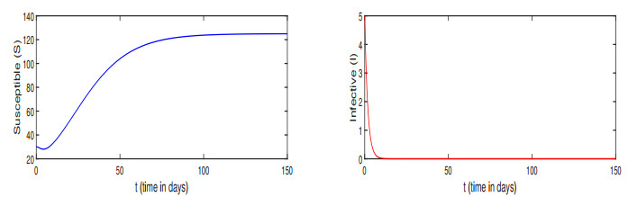
A delay differential equation model of an infectious disease is considered and analyzed. In this model, the impact of information due to the presence of infection is considered explicitly. As information propagation is dependent on the prevalence of the disease, the delay in reporting the prevalence is an important factor. Further, the time lag in waning immunity related to protective measures (such as vaccination, self-protection, responsive behaviour etc.) is also accounted. Qualitative analysis of the equilibrium points of the model is executed and it is observed that when the basic reproduction number is less unity, the local stability of the disease free equilibrium (DFE) depends on the rate of immunity loss as well as on the time delay for the waning of immunity. If the delay in immunity loss is less than a threshold quantity, the DFE is stable, whereas, it loses its stability when the delay parameter crosses the threshold value. When, the basic reproduction number is greater than unity, the unique endemic equilibrium point is found locally stable irrespective of the delay effect under certain parametric conditions. Further, we have analyzed the model system for different scenarios of both delays (i.e., no delay, only one delay, and both delay present). Due to these delays, oscillatory nature of the population is obtained with the help of Hopf bifurcation analysis in each scenario. Moreover, at two different time delays (delay in information's propagation), the emergence of multiple stability switches is investigated for the model system which is termed as Hopf-Hopf (double) bifurcation. Also, the global stability of the endemic equilibrium point is established under some parametric conditions by constructing a suitable Lyapunov function irrespective of time lags. In order to support and explore qualitative results, exhaustive numerical experimentations are carried out which lead to important biological insights and also, these results are compared with existing results.
Citation: Anuj Kumar, Yasuhiro Takeuchi, Prashant K Srivastava. Stability switches, periodic oscillations and global stability in an infectious disease model with multiple time delays[J]. Mathematical Biosciences and Engineering, 2023, 20(6): 11000-11032. doi: 10.3934/mbe.2023487
A delay differential equation model of an infectious disease is considered and analyzed. In this model, the impact of information due to the presence of infection is considered explicitly. As information propagation is dependent on the prevalence of the disease, the delay in reporting the prevalence is an important factor. Further, the time lag in waning immunity related to protective measures (such as vaccination, self-protection, responsive behaviour etc.) is also accounted. Qualitative analysis of the equilibrium points of the model is executed and it is observed that when the basic reproduction number is less unity, the local stability of the disease free equilibrium (DFE) depends on the rate of immunity loss as well as on the time delay for the waning of immunity. If the delay in immunity loss is less than a threshold quantity, the DFE is stable, whereas, it loses its stability when the delay parameter crosses the threshold value. When, the basic reproduction number is greater than unity, the unique endemic equilibrium point is found locally stable irrespective of the delay effect under certain parametric conditions. Further, we have analyzed the model system for different scenarios of both delays (i.e., no delay, only one delay, and both delay present). Due to these delays, oscillatory nature of the population is obtained with the help of Hopf bifurcation analysis in each scenario. Moreover, at two different time delays (delay in information's propagation), the emergence of multiple stability switches is investigated for the model system which is termed as Hopf-Hopf (double) bifurcation. Also, the global stability of the endemic equilibrium point is established under some parametric conditions by constructing a suitable Lyapunov function irrespective of time lags. In order to support and explore qualitative results, exhaustive numerical experimentations are carried out which lead to important biological insights and also, these results are compared with existing results.

| [1] | F. Brauer, C. Castillo-Chavez, Mathematical Models in Population Biology and Epidemiology, Springer, 2001. |
| [2] | O. Diekmann, J. A. P. Heesterbeek, Mathematical Epidemiology of Infectious Diseases: Model Building, Analysis and Interpretation, John Wiley & Sons, 2000. |
| [3] |
H. W. Hethcote, The mathematics of infectious diseases, SIAM Rev., 42 (2000), 599–653. https://doi.org/10.1137/S0036144500371907 doi: 10.1137/S0036144500371907

|
| [4] |
W. O. Kermack, A. G. McKendrick, A contribution to the mathematical theory of epidemics, Proc. R. Soc. Lond. A, 115 (1927), 700–721. https://doi.org/10.1098/rspa.1927.0118 doi: 10.1098/rspa.1927.0118
|
| [5] |
M. E. Alexander, C. Bowman, S. M. Moghadas, R. Summers, A. B. Gumel, B. M. Sahai, A vaccination model for transmission dynamics of influenza, SIAM J. Appl. Dyn. Syst., 3 (2004), 503–524. https://doi.org/10.1137/03060037 doi: 10.1137/03060037
|
| [6] |
A. B. Gumel, S. Ruan, T. Day, J. Watmough, F. Brauer, P. van den Driessche, et al., Modelling strategies for controlling SARS outbreaks, Proc. R. Soc. B: Biol. Sci., 271 (2004), 2223–2232. https://doi.org/10.1098/rspb.2004.2800 doi: 10.1098/rspb.2004.2800
|
| [7] |
S. Lee, G. Chowell, C. Castillo-Chávez, Optimal control for pandemic influenza: the role of limited antiviral treatment and isolation, J. Theor. Biol., 265 (2010), 136–150. https://doi.org/10.1016/j.jtbi.2010.04.003 doi: 10.1016/j.jtbi.2010.04.003
|
| [8] |
X. Liu, Y. Takeuchi, S. Iwami, SVIR epidemic models with vaccination strategies, J. Theor. Biol., 253 (2008), 1–11. https://doi.org/10.1016/j.jtbi.2007.10.014 doi: 10.1016/j.jtbi.2007.10.014
|
| [9] |
Z. Qiu, Z. Feng, Transmission dynamics of an influenza model with vaccination and antiviral treatment, Bull. Math. Biol., 72 (2010), 1–33. https://doi.org/10.1007/s11538-009-9435-5 doi: 10.1007/s11538-009-9435-5
|
| [10] |
A. Kumar, P. K. Srivastava, Vaccination and treatment as control interventions in an infectious disease model with their cost optimization, Commun. Nonlinear Sci. Numer. Simul., 44 (2017), 334–343. https://doi.org/10.1016/j.cnsns.2016.08.005 doi: 10.1016/j.cnsns.2016.08.005
|
| [11] |
A. Kumar, P. K. Srivastava, Y. Takeuchi, Modeling the role of information and limited optimal treatment on disease prevalence, J. Theor. Biol., 414 (2017), 103–119. https://doi.org/10.1016/j.jtbi.2016.11.016 doi: 10.1016/j.jtbi.2016.11.016
|
| [12] |
Y. Yuan, N. Li, Optimal control and cost-effectiveness analysis for a COVID-19 model with individual protection awareness, Phys. A: Stat. Mech. Appl., 603 (2022), 127804. https://doi.org/10.1016/j.physa.2022.127804 doi: 10.1016/j.physa.2022.127804
|
| [13] |
P. A. Gonz$\acute{a}$lez-Parra, S. Lee, L. Velazquez, C. Castillo-Chavez, A note on the use of optimal control on a discrete time model of influenza dynamics, Math. Biosci. Eng., 8 (2011), 183–197. doi: 10.3934/mbe.2011.8.183 doi: 10.3934/mbe.2011.8.183
|
| [14] |
S. M. Kassa, A. Ouhinou, The impact of self-protective measures in the optimal interventions for controlling infectious diseases of human population, J. Math. Biol., 70 (2015), 213–236. https://doi.org/10.1007/s00285-014-0761-3 doi: 10.1007/s00285-014-0761-3
|
| [15] |
A. Kumar, P. K. Srivastava, Y. Dong, Y. Takeuchi, Optimal control of infectious disease: Information-induced vaccination and limited treatment, Physica A: Stat. Mech. Appl., 542 (2020), 123196. https://doi.org/10.1016/j.physa.2019.123196 doi: 10.1016/j.physa.2019.123196
|
| [16] |
A. Yadav, P. K. Srivastava, A. Kumar, Mathematical model for smoking: Effect of determination and education, Int. J. Biomath., 8 (2015), 1550001. https://doi.org/10.1142/S1793524515500011 doi: 10.1142/S1793524515500011
|
| [17] | World Health Organization (WHO), Government of Senegal boosts Ebola awareness through SMS campaign, 2014. Avaliable from: http://http://www.who.int/features/2014/senegal-ebola-sms/en/. |
| [18] |
A. Ahituv, V. J. Hotz, T. Philipson, The responsiveness of the demand for condoms to the local prevalence of AIDS, J. Hum. Resour., 31 (1996), 869–897. https://doi.org/10.2307/146150 doi: 10.2307/146150
|
| [19] |
D. Greenhalgh, S. Rana, S. Samanta, T. Sardar, S. Bhattacharya, J. Chattopadhyay, Awareness programs control infectious disease-multiple delay induced mathematical model, Appl. Math. Comput., 251 (2015), 539–563. https://doi.org/10.1016/j.amc.2014.11.091 doi: 10.1016/j.amc.2014.11.091
|
| [20] |
Y. Liu, J. Cui, The impact of media coverage on the dynamics of infectious disease, Int. J. Biomath., 1 (2008), 65–74. https://doi.org/10.1142/S1793524508000023 doi: 10.1142/S1793524508000023
|
| [21] |
A. K. Misra, A. Sharma, V. Singh, Effect of awareness programs in controlling the prevalence of an epidemic with time delay. J. Biol. Syst., 19 (2011), 389–402. https://doi.org/10.1142/S0218339011004020 doi: 10.1142/S0218339011004020
|
| [22] |
T. Philipson, Private vaccination and public health: an empirical examination for US measles, J. Hum. Resour., 31 (1996), 611–630. https://doi.org/10.2307/146268 doi: 10.2307/146268
|
| [23] |
J. Cui, Y. Sun, H. Zhu, The impact of media on the control of infectious diseases, J. Dyn. Differ. Equations, 20 (2008), 31–53. https://doi.org/10.1007/s10884-007-9075-0 doi: 10.1007/s10884-007-9075-0
|
| [24] |
A. d'Onofrio, P. Manfredi, Information-related changes in contact patterns may trigger oscillations in the endemic prevalence of infectious diseases, J. Theor. Biol., 256 (2009), 473–478. https://doi.org/10.1016/j.jtbi.2008.10.005 doi: 10.1016/j.jtbi.2008.10.005
|
| [25] |
S. Funk, E. Gilad, C. Watkins, V. A. A. Jansen, The spread of awareness and its impact on epidemic outbreaks, Proc. Natl. Acad. Sci. U.S.A., 106 (2009), 6872–6877. https://doi.org/10.1073/pnas.08107621 doi: 10.1073/pnas.08107621
|
| [26] |
I. Z. Kiss, J. Cassell, M. Recker, P. L. Simon, The impact of information transmission on epidemic outbreaks, Math. Biosci., 225 (2010), 1–10. https://doi.org/10.1016/j.mbs.2009.11.009 doi: 10.1016/j.mbs.2009.11.009
|
| [27] |
Y. Li, C. Ma, J. Cui, The effect of constant and mixed impulsive vaccination on SIS epidemic models incorporating media coverage, Rocky Mt. J. Math., 38 (2008), 1437–1455. DOI: 10.1216/RMJ-2008-38-5-1437 doi: 10.1216/RMJ-2008-38-5-1437
|
| [28] |
R. Liu, J. Wu, H. Zhu, Media/psychological impact on multiple outbreaks of emerging infectious diseases, Comput. Math. Methods Med., 8 (2007), 153–164. https://doi.org/10.1080/17486700701425870 doi: 10.1080/17486700701425870
|
| [29] | P. Manfredi, A. d'Onofrio, Modeling the Interplay Between Human Behavior and the Spread of Infectious Diseases, Springer Science & Business Media, 2013. |
| [30] |
K. Cooke, P. Van. den Driessche, X. Zou, Interaction of maturation delay and nonlinear birth in population and epidemic models, J. Math. Biol., 39 (1999), 332–352. https://doi.org/10.1007/s002850050194 doi: 10.1007/s002850050194
|
| [31] |
D. Greenhalgh, Q. J. A. Khan, F. I. Lewis, Recurrent epidemic cycles in an infectious disease model with a time delay in loss of vaccine immunity, Nonlinear Anal. Theory Methods Appl., 63 (2005), e779–e788. https://doi.org/10.1016/j.na.2004.12.018 doi: 10.1016/j.na.2004.12.018
|
| [32] |
G. Huang, Y. Takeuchi, W. Ma, D. Wei, Global stability for delay SIR and SEIR epidemic models with nonlinear incidence rate, Bull. Math. Biol., 72 (2010), 1192–1207. https://doi.org/10.1007/s11538-009-9487-6 doi: 10.1007/s11538-009-9487-6
|
| [33] | Y. Kuang, Delay Differential Equations: with Applications in Population Dynamics, Academic Press, 1993. |
| [34] |
N. Kyrychko, K. B. Blyuss, Global properties of a delayed SIR model with temporary immunity and nonlinear incidence rate, Nonlinear Anal. Real World Appl., 6 (2005), 495–507. https://doi.org/10.1016/j.nonrwa.2004.10.001 doi: 10.1016/j.nonrwa.2004.10.001
|
| [35] |
M. Liu, E. Liz, G. Röst, Endemic bubbles generated by delayed behavioral response: global stability and bifurcation switches in an SIS model, SIAM J. Appl. Math., 75 (2015), 75–91. https://doi.org/10.1137/140972652 doi: 10.1137/140972652
|
| [36] |
Y. Song, J. Wei, Bifurcation analysis for chen's system with delayed feedback and its application to control of chaos, Chaos, Solitons Fractals, 22 (2004), 75–91. https://doi.org/10.1016/j.chaos.2003.12.075 doi: 10.1016/j.chaos.2003.12.075
|
| [37] |
L. Wen, X. Yang, Global stability of a delayed SIRS model with temporary immunity, Chaos, Solitons Fractals, 38 (2008), 221–226. https://doi.org/10.1016/j.chaos.2006.11.010 doi: 10.1016/j.chaos.2006.11.010
|
| [38] |
T. Cheng, X. Zou, A new perspective on infection forces with demonstration by a DDE infectious disease model, Math. Biosci. Eng., 19 (2022), 4856–4880. doi: 10.3934/mbe.2022227 doi: 10.3934/mbe.2022227
|
| [39] |
A. d'Onofrio, P. Manfredi, E. Salinelli, Vaccinating behaviour, information, and the dynamics of SIR vaccine preventable diseases, Theor. Popul. Biol., 71 (2007), 301–317. https://doi.org/10.1016/j.tpb.2007.01.001 doi: 10.1016/j.tpb.2007.01.001
|
| [40] |
P. K. Srivastava, M. Banerjee, P. Chandra, A primary infection model for HIV and immune response with two discrete time delays, Differ. Equations Dyn. Syst., 18 (2010), 385–399. https://doi.org/10.1007/s12591-010-0074-y doi: 10.1007/s12591-010-0074-y
|
| [41] |
P. K. Srivastava, P. Chandra, Hopf bifurcation and periodic solutions in a dynamical model for HIV and immune response, Differ. Equations Dyn. Syst., 16 (2008), 77–100. https://doi.org/10.1007/s12591-008-0006-2 doi: 10.1007/s12591-008-0006-2
|
| [42] |
H. Zhao, Y. Lin, Y. Dai, An SIRS epidemic model incorporating media coverage with time delay, Comput. Math. Methods Med., 2014 (2014). https://doi.org/10.1155/2014/680743 doi: 10.1155/2014/680743
|
| [43] |
Z. Lv, X. Liu, Y. Ding, Dynamic behavior analysis of an SVIR epidemic model with two time delays associated with the COVID-19 booster vaccination time, Math. Biosci. Eng., 20 (2023), 6030–6061. https://doi.org/10.3934/mbe.2023261 doi: 10.3934/mbe.2023261
|
| [44] |
Y. Ma, Y. Cui, M. Wang, Global stability and control strategies of a SIQRS epidemic model with time delay, Math. Methods Appl. Sci., 45 (2022), 8269–8293. https://doi.org/10.1002/mma.8309 doi: 10.1002/mma.8309
|
| [45] |
A. Mezouaghi, S. Djillali, A. Zeb, K.S. Nisar, Global proprieties of a delayed epidemic model with partial susceptible protection, Math. Biosci. Eng., 19 (2022), 209–224. https://doi.org/10.3934/mbe.2022011 doi: 10.3934/mbe.2022011
|
| [46] |
H. Yang, Y. Wang, S. Kundu, Z. Song, Z. Zhang, Dynamics of an SIR epidemic model incorporating time delay and convex incidence rate, Results Phys., 32 (2022), 105025. https://doi.org/10.1016/j.rinp.2021.105025 doi: 10.1016/j.rinp.2021.105025
|
| [47] |
A. Kumar, P. K. Srivastava, A. Yadav, Delayed information induces oscillations in a dynamical model for infectious disease, Int. J. Biomath., 12 (2019), 1950020. https://doi.org/10.1142/S1793524519500207 doi: 10.1142/S1793524519500207
|
| [48] |
M. V. Barbarossa, M. Polner, G. Röst, Stability switches induced by immune system boosting in an sirs model with discrete and distributed delays, SIAM J. Appl. Math., 77 (2017), 905–923. https://doi.org/10.1137/16M1077234 doi: 10.1137/16M1077234
|
| [49] |
M. V. Barbarossa, G. Röst, Immuno-epidemiology of a population structured by immune status: a mathematical study of waning immunity and immune system boosting, J. Math. Biol., 71 (2015), 1737–1770. https://doi.org/10.1007/s00285-015-0880-5 doi: 10.1007/s00285-015-0880-5
|
| [50] | D. Wodarz, Killer Cell Dynamics: Mathematical and Computational Approaches to Immunology, Springer, 2007. |
| [51] |
Q. An, E. Beretta, Y. Kuang, C. Wang, H. Wang, Geometric stability switch criteria in delay differential equations with two delays and delay dependent parameters, J. Differ. Equations, 266 (2019), 7073–7100. https://doi.org/10.1016/j.jde.2018.11.025 doi: 10.1016/j.jde.2018.11.025
|
| [52] | X. Lin, H. Wang, Stability analysis of delay differential equations with two discrete delays, Can. Appl. Math. Q., 20 (2012), 519–533. |
| [53] |
D. Li, B. Chai, W. Liu, P. Wen, R. Zhang, Qualitative analysis of a class of SISM epidemic model influenced by media publicity, Math. Biosci. Eng., 17 (2020), 5727–5751. https://doi.org/10.3934/mbe.2020308 doi: 10.3934/mbe.2020308
|
| [54] |
A. Yadav, P. K. Srivastava, The impact of information and saturated treatment with time delay in an infectious disease model, J. Appl. Math. Comput., 66 (2021), 277–305. https://doi.org/10.1007/s12190-020-01436-2 doi: 10.1007/s12190-020-01436-2
|
| [55] |
Z. Zhang, G. ur Rahman, J. F. Gómez-Aguilar, J. Torres-Jiménez, Dynamical aspects of a delayed epidemic model with subdivision of susceptible population and control strategies, Chaos, Solitons Fractals, 160 (2022), 112194. https://doi.org/10.1016/j.chaos.2022.112194 doi: 10.1016/j.chaos.2022.112194
|
| [56] |
H. Zhao, M. Zhao, Global hopf bifurcation analysis of an susceptible-infective-removed epidemic model incorporating media coverage with time delay, J. Biol. Dyn., 11 (2017), 8–24. https://doi.org/10.1080/17513758.2016.1229050 doi: 10.1080/17513758.2016.1229050
|
| [57] |
Y. Liu, J. Wei, Bifurcation analysis in delayed nicholson blowflies equation with delayed harvest, Nonlinear Dyn., 105 (2021), 1805–1819. https://doi.org/10.1007/s11071-021-06651-5 doi: 10.1007/s11071-021-06651-5
|
| [58] | S. Ruan, J. Wei, On the zeros of transcendental functions with applications to stability of delay differential equations with two delays, Dyn. Contin. Discrete Impuls. Syst. A: Math. Anal., 10 (2003), 863–874. |
| [59] |
X. Wang, A simple proof of descartes's rule of signs, Am. Math. Mon., 111 (2004), 525. https://doi.org/10.1080/00029890.2004.11920108 doi: 10.1080/00029890.2004.11920108
|
| [60] |
H. I. Freedman, V. S. H. Rao, The trade-off between mutual interference and time lags in predator-prey systems, Bull. Math. Biol., 45 (1983), 991–1004. https://doi.org/10.1016/S0092-8240(83)80073-1 doi: 10.1016/S0092-8240(83)80073-1
|
| [61] | J. K. Hale, Functional Differential Equations, Springer, New York, 1977. |
| [62] | J. P. La Salle, The Stability of Dynamical Systems, Society for Industrial and Applied Mathematics, SIAM, Philadelphia, 1976. |
| [63] |
H. Jiang, T. Zhang, Y. Song, Delay-induced double hopf bifurcations in a system of two delay-coupled van der pol-duffing oscillators, Int. J. Bifurcation Chaos, 25 (2015), 1550058. https://doi.org/10.1142/S0218127415500583 doi: 10.1142/S0218127415500583
|
| [64] |
H. Zang, T. Zhang, Y. Zhang, Stability and bifurcation analysis of delay coupled van der pol-duffing oscillators, Nonlinear Dyn., 75 (2014), 35–47. https://doi.org/10.1007/s11071-013-1047-9 doi: 10.1007/s11071-013-1047-9
|
| [65] |
M. Adimy, F. Crauste, S. Ruan, Periodic oscillations in leukopoiesis models with two delays, J. Theor. Biol., 242 (2006), 288–299. https://doi.org/10.1016/j.jtbi.2006.02.020 doi: 10.1016/j.jtbi.2006.02.020
|


Figures(20)

Anuj Kumar, Yasuhiro Takeuchi, Prashant K Srivastava. Stability switches, periodic oscillations and global stability in an infectious disease model with multiple time delays[J]. Mathematical Biosciences and Engineering, 2023, 20(6): 11000-11032. doi: 10.3934/mbe.2023487


 DownLoad: