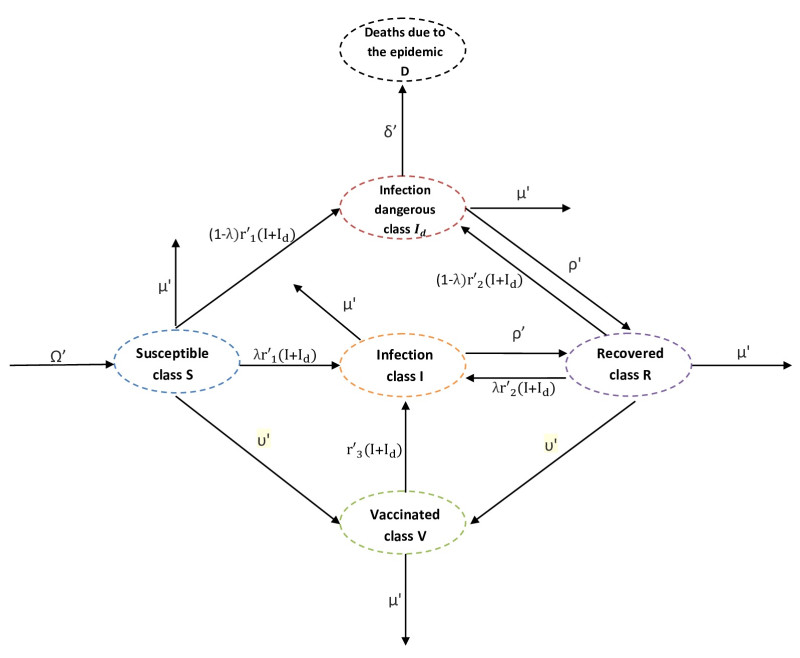
Referring tothe study of epidemic mathematical models, this manuscript presents a noveldiscrete-time COVID-19 model that includes the number of vaccinated individuals as an additional state variable in the system equations. The paper shows that the proposed compartment model, described by difference equations, has two fixed points, i.e., a disease-free fixed point and an epidemic fixed point. By considering both the forward difference system and the backward difference system, some stability analyses of the disease-free fixed point are carried out.In particular, for the backward difference system a novel theorem is proved, which gives a condition for the disappearance of the pandemic when an inequality involving some epidemic parameters is satisfied. Finally, simulation results of the conceived discrete model are carried out, along with comparisons regarding the performances of both the forward difference system and the backward difference system.
Citation: A Othman Almatroud, Noureddine Djenina, Adel Ouannas, Giuseppe Grassi, M Mossa Al-sawalha. A novel discrete-time COVID-19 epidemic model including the compartment of vaccinated individuals[J]. Mathematical Biosciences and Engineering, 2022, 19(12): 12387-12404. doi: 10.3934/mbe.2022578
Referring tothe study of epidemic mathematical models, this manuscript presents a noveldiscrete-time COVID-19 model that includes the number of vaccinated individuals as an additional state variable in the system equations. The paper shows that the proposed compartment model, described by difference equations, has two fixed points, i.e., a disease-free fixed point and an epidemic fixed point. By considering both the forward difference system and the backward difference system, some stability analyses of the disease-free fixed point are carried out.In particular, for the backward difference system a novel theorem is proved, which gives a condition for the disappearance of the pandemic when an inequality involving some epidemic parameters is satisfied. Finally, simulation results of the conceived discrete model are carried out, along with comparisons regarding the performances of both the forward difference system and the backward difference system.

| [1] |
H. W. Hethcote, The mathematics of infectious diseases, SIAM Rev., 42 (2000), 599–653. https://doi.org/10.1137/S0036144500371907 doi: 10.1137/S0036144500371907

|
| [2] |
T. T. Marinov, R. S. Marinova, Dynamics of COVID-19 using inverse problem for coefficient identification in SIR epidemic models, Chaos Solit. Fract., 5 (2020). https://doi.org/10.1016/j.csfx.2020.100041 doi: 10.1016/j.csfx.2020.100041
|
| [3] |
J. T. Wu, K. Leung, M. Bushman, N. Kishore, R. Niehus, P. M. de Salazar, et al., Estimating clinical severity of COVID-19 from the transmission dynamics in Wuhan, China, Nat. Med., 26 (2020), 506–510. https://doi.org/10.1038/s41591-020-0822-7 doi: 10.1038/s41591-020-0822-7
|
| [4] |
S. Mangiarotti, M. Peyre, Y. Zhang, M. Huc, F. Roger, Y. Kerr, Chaos theory applied to the outbreak of COVID-19: An ancillary approach to decision making in pandemic context, Epidem. Infect, 148 (2020), 1–29. https://doi.org/10.1017/S0950268820000990 doi: 10.1017/S0950268820000990
|
| [5] |
S. Gounane, Y. Barkouch, A. Atlas, M. Bendahmane, F. Karami, D. Meskine, An adaptive social distancing SIR model for COVID-19 disease spreading and forecasting, Epidem. Methods, 10 (2021), 20200044. https://doi.org/10.1515/em-2020-0044 doi: 10.1515/em-2020-0044
|
| [6] |
G. Giordano, F. Blanchini, R. Bruno, P. Colaneri, A. Di Filippo, A. Di Matteo, et al., Modelling the COVID-19 epidemic and implementation of population-wide interventions in Italy, Nat. Med., 26 (2020), 855–860. https://doi.org/10.1038/s41591-020-0883-7 doi: 10.1038/s41591-020-0883-7
|
| [7] |
A. Ajbar, R. T. Alqahtani, M. Boumaza1, Dynamics of an SIR-Based COVID-19 Model With Linear Incidence Rate, Nonlinear Removal Rate, and Public Awareness, Front. Phys., (2021). https://doi.org/10.3389/fphy.2021.634251 doi: 10.3389/fphy.2021.634251
|
| [8] |
P. Kumara, V. S. Erturk, M. Murillo-Arcila, A new fractional mathematical modelling of COVID-19 with the availability of vaccine, Results Phys., 24 (2021), 2211–3797. https://doi.org/10.1016/j.rinp.2021.104213 doi: 10.1016/j.rinp.2021.104213
|
| [9] |
N. Gozalpour, E. Badfar, A. Nikoofard, Transmission dynamics of novel coronavirus SARS-CoV-2 among healthcare workers, a case study in Iran, Nonlinear Dynam., 105 (2021), 3749–-3761. https://doi.org/10.1007/s11071-021-06778-5 doi: 10.1007/s11071-021-06778-5
|
| [10] |
E. Badfar, E. J. Zaferani, A. Nikoofard, Design a robust sliding mode controller based on the state and parameter estimation for the nonlinear epidemiological model of Covid-19, Nonlinear Dynam., (2021), 5–-18. https://doi.org/10.1007/s11071-021-07036-4 doi: 10.1007/s11071-021-07036-4
|
| [11] |
A. Rajaei, M. Raeiszadeh, V. Azimi, M. Sharifi, State estimation-based control of COVID-19 epidemic before and after vaccine development, J. Pro. Control, 102 (2021), 1–14. https://doi.org/10.1016/j.jprocont.2021.03.008 doi: 10.1016/j.jprocont.2021.03.008
|
| [12] |
M. De la Sen, A. Ibeas, R. Nistal, About partial reachability issues in an SEIR epidemic model and related infectious disease tracking in finite time under vaccination and treatment controls, Discrete Dynam. Nat. Soc., (2021). https://doi.org/10.1155/2021/5556897 doi: 10.1155/2021/5556897
|
| [13] |
M. De la Sen, A. Ibeas, On an SE(Is)(Ih)AR epidemic model with combined vaccination and antiviral controls for COVID-19 pandemic, Adv. Difference Equ., 92 (2021). https://doi.org/10.1186/s13662-021-03248-5 doi: 10.1186/s13662-021-03248-5
|
| [14] |
S. Zhai, G. Luo, T. Huang, X. Wang, J. Tao, P. Zhou, Vaccination control of an epidemic model with time delay and its application to COVID-19, Nonlinear Dynam., 106 (2021), 1279–1292. https://doi.org/10.1007/s11071-021-06533-w doi: 10.1007/s11071-021-06533-w
|
| [15] |
E. Hwang, Prediction intervals of the COVID-19 cases by HAR models with growth rates and vaccination rates in top eight affected countries: Bootstrap improvement, Chaos Solit. Fract., 155 (2022). https://doi.org/10.1016/j.chaos.2021.111789 doi: 10.1016/j.chaos.2021.111789
|
| [16] |
P. Mahmood, M. Saeed, Stability of the equilibria in a discrete-time sivs epidemic model with standard incidence, Filomat, 33 (2019), 2393–2408. https://doi.org/10.1016/j.chaos.2021.111789 doi: 10.1016/j.chaos.2021.111789
|
| [17] |
M. De la Sen, S. Alonso-Quesada, A. Ibeas, On a Discrete SEIR Epidemic Model with Exposed Infectivity, Feedback Vaccination and Partial Delayed Re-Susceptibility, Mathematics, 9 (2021), 5–9. https://doi.org/10.3390/math9050520 doi: 10.3390/math9050520
|
| [18] |
M. De la Sen, S. Alonso-Quesada, A. Ibeas, R. Nistal, On a Discrete SEIR Epidemic Model with Two-Doses Delayed Feedback Vaccination Control on the Susceptible, Vaccines, 9 (2021). https://doi.org/10.3390/vaccines9040398 doi: 10.3390/vaccines9040398
|
| [19] |
Y. Omae, Y. Kakimoto, M. Sasaki, J. Toyotani, K. Hara, Y. Gon, et al., SIRVVD model-based verification of the effect of first and second doses of COVID-19/SARS-CoV-2 vaccination in Japan, Math. Biosci. Eng., 19 (2021), 1026–1040. https://doi.org/10.3934/mbe.2022047 doi: 10.3934/mbe.2022047
|
| [20] | N. Djenina, I. Rezzoug, A. Ouannas, T-E. Oussaeif, Giuseppe Grassi, A new COVID-19 pandemic model including the compartment of vaccinated individuals: Global stability of the disease-free fixed point, Submitted to CMMM, 2022 (2022). |
| [21] |
P. van den Driesschea, J. Watmough, Reproduction numbers and sub-threshold endemic equilibria for compartmental models of disease transmission, Math. Biosci., 180 (2002). https://doi.org/10.1016/S0025-5564(02)00108-6 doi: 10.1016/S0025-5564(02)00108-6
|
| [22] |
S. Elaydi, An introduction to difference equations, Springer SBM, 3 (2005). https://doi.org/10.1007/0-387-27602-5 doi: 10.1007/0-387-27602-5
|
Figures(5)

A Othman Almatroud, Noureddine Djenina, Adel Ouannas, Giuseppe Grassi, M Mossa Al-sawalha. A novel discrete-time COVID-19 epidemic model including the compartment of vaccinated individuals[J]. Mathematical Biosciences and Engineering, 2022, 19(12): 12387-12404. doi: 10.3934/mbe.2022578


 DownLoad: