Open set recognition algorithm based on Conditional Gaussian Encoder

Yan Tang; Zhijin Zhao; Chun Li; Xueyi Ye; Yan Tang; Zhijin Zhao; Chun Li; Xueyi Ye

doi:10.3934/mbe.2021328

Mathematical Biosciences and Engineering

2021, Volume 18, Issue 5: 6620-6637. doi: 10.3934/mbe.2021328

Previous Article Next Article

Research article Special Issues

Open set recognition algorithm based on Conditional Gaussian Encoder

1.
School of Communication Engineering, Hangzhou Dianzi University, Hangzhou, China
2.
State Key Lab of Information Control Technology in Communication System, The 36th Research Institute of China Electronics Technology Group Corporation, Jiaxing, China

Received: 08 July 2021 Accepted: 01 August 2021 Published: 03 August 2021

For the existing Closed Set Recognition (CSR) methods mistakenly identify unknown jamming signals as a known class, a Conditional Gaussian Encoder (CG-Encoder) for 1-dimensional signal Open Set Recognition (OSR) is designed. The network retains the original form of the signal as much as possible and deep neural network is used to extract useful information. CG-Encoder adopts residual network structure and a new Kullback-Leibler (KL) divergence is defined. In the training phase, the known classes are approximated to different Gaussian distributions in the latent space and the discrimination between classes is increased to improve the recognition performance of the known classes. In the testing phase, a specific and effective OSR algorithm flow is designed. Simulation experiments are carried out on 9 jamming types. The results show that the CSR and OSR performance of CG-Encoder is better than that of the other three kinds of network structures. When the openness is the maximum, the open set average accuracy of CG-Encoder is more than 70%, which is about 30% higher than the worst algorithm, and about 20% higher than the better one. When the openness is the minimum, the average accuracy of OSR is more than 95%.
- Jamming recognition,
- Open Set Recognition (OSR),
- Conditional Gaussian Encoder (CG-Encoder),
- residual network,
- Kullback-Leibler (KL) divergence
Citation: Yan Tang, Zhijin Zhao, Chun Li, Xueyi Ye. Open set recognition algorithm based on Conditional Gaussian Encoder[J]. Mathematical Biosciences and Engineering, 2021, 18(5): 6620-6637. doi: 10.3934/mbe.2021328

Related Papers:

Abstract

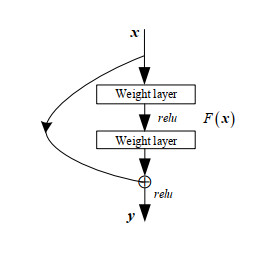
For the existing Closed Set Recognition (CSR) methods mistakenly identify unknown jamming signals as a known class, a Conditional Gaussian Encoder (CG-Encoder) for 1-dimensional signal Open Set Recognition (OSR) is designed. The network retains the original form of the signal as much as possible and deep neural network is used to extract useful information. CG-Encoder adopts residual network structure and a new Kullback-Leibler (KL) divergence is defined. In the training phase, the known classes are approximated to different Gaussian distributions in the latent space and the discrimination between classes is increased to improve the recognition performance of the known classes. In the testing phase, a specific and effective OSR algorithm flow is designed. Simulation experiments are carried out on 9 jamming types. The results show that the CSR and OSR performance of CG-Encoder is better than that of the other three kinds of network structures. When the openness is the maximum, the open set average accuracy of CG-Encoder is more than 70%, which is about 30% higher than the worst algorithm, and about 20% higher than the better one. When the openness is the minimum, the average accuracy of OSR is more than 95%.

References

[1]	F. Q. Yao, Communication anti-jamming engineering and practice, Beijing Publishing House Electron. Industry, (2008), 1-8.
[2]	Y. Y. Wen, J. Y. Wei, H. Chen, A new algorithm of interferences signals recognition, Space Electron. Technol., 1 (2015), 85-88.
[3]	J. X. Wang, Q. Chang, Y. Tian, J. Huang, Research on GNSS interference signal detection method, Navig. Position. Tim., 4 (2020), 117-122.
[4]	G. S. Wang, Q. H. Ren, Z. G. Jang, Y. Liu, B. Z. Xu, Jamming classification and recognition in transform domain communication system based on signal feature space, Syst. Eng. Electron., 39 (2017), 1950-1958.
[5]	G. C. Huang, G. S. Wang, Q. H. Ren, S. F. Dong, W. T. Gao, S. Wei, Adaptive recognition method for unknown interference based on Hilbert signal space, J. Electron. Inform. Technol., 41 (2017), 1916-1923.
[6]	J. Y. Liu, Research on electronic jamming identification method based on time frequency domain analysis, University Electron. Sci. Technol. China, 2018.
[7]	G. J. Xun, Research on identification of typical communication jamming signals, University Electron. Sci. Technol. China, 2018.
[8]	Q. Liu, W. Zhang, Deep learning and recognition of radar jamming based on CNN, 2019 12th International Symposium on Computational Intelligence and Design (ISCID), IEEE, 1 (2019), 208-212.
[9]	T. F. Chi, Recognition algorithm for the four kinds of interference signals, Huazhong University Sci. Technol., 2019.
[10]	Z. B. Zhang, Y. X. Fan, X. Meng, Pattern recognition method of communication interference based on power spectrum density and neural network, J. Terahertz Sci. Electron. Inform. Technol., 17 (2019), 959-963.
[11]	Y. Cai, K. Shi, F. Song, Y. F. Xu, X. M. Wang, H. Y. Luan, Jamming pattern recognition using spectrum waterfall. a deep learning method, 2019 IEEE 5th International Conference on Computer and Communications (ICCC), IEEE, (2019), 2113-2117.
[12]	Z. L. Wu, Y. L. Zhao, Z. D. Yin, H. C. Luo, Jamming signals classification using convolutional neural network, 2017 IEEE International Symposium on Signal Processing and Information Technology (ISSPIT), IEEE, (2017), 062-067.
[13]	W. J. Scheirer, A. R. Rocha, A. Sapkota, T. E. Boult, Towards open set recognition, IEEE Transact. Pattern Anal. Mach. Intell., 35 (2013), 1757-1772.
[14]	M. D. Scherreik, B. D. Rigling, Open set recognition for automatic target classification with rejection, IEEE Transact. Aerosp. Electron. Systems, 52 (2016), 632-642. doi: 10.1109/TAES.2015.150027
[15]	P. R. M. Jnior, R. M. D. Souza, R. D. O. Werneck, B. V. Stein, D.V. Pazinato, W. R. Almeida, et al, Nearest neighbors distance ratio open-set classifier, Mach. Learn., 106 (2017), 359-386.
[16]	E. M. Rudd, L. P. Jain, W. J. Scheirer, T. E. Boult, The extreme value machine, IEEE Transact. Pattern Anal. Mach. Intell., 40 (2018), 762-768.
[17]	E. Vignotto, S. Engelke, Extreme value theory for open set classification GPD and GEV classifiers, arXiv preprint, arXiv: 1808.09902, 2018.
[18]	K. He, X. Zhang, S. Ren, J. Sun, Deep residual learning for image recognition, Proceedings of the IEEE Conference on Computer Vision and Pattern Recognition, (2016), 770-778.
[19]	A Bendale, T. E. Boult, Towards open set deep networks, Proceedings of the IEEE Conference on Computer Vision and Pattern Recognition, (2016), 1563-1572.
[20]	S. Prakhya, V. Venkataram, J. Kalita, Open set text classification using convolutional neural networks, International Conference on Natural Language Processing, 2017.
[21]	L. Shu, H. Xu, B. Liu, DOC: Deep open classification of text documents, Proceedings of the 2017 Conference on Empirical Methods in Natural Language Processing, (2017), 2911-2916.
[22]	N. Kardan, K. O. Stanley, Mitigating fooling with competitive overcomplete output layer neural networks, International Joint Conference on Neural Networks (IJCNN), (2017), 518-525.
[23]	A. R. Dhamija, M. Günther, T. Boult, Reducing network agnostophobia, Advances in Neural Information Processing Systems, (2018), 9157-9168.
[24]	L. Shu, H. Xu, B. Liu, Unseen class discovery in open-world classification, arXiv preprint, arXiv: 1801.05609, 2018.
[25]	I. Goodfellow, J. P. Abadie, M. Mirza, B. Xu, D. W. Farley, S. Ozair, et al., Generative adversarial nets, Adv. Neural Inform. Process. Systems, (2014), 2672-2680.
[26]	X. Sun, Z. N. Yang, C. Zhang, Xin Sun, K. V. Ling, G. H. Peng, Conditional gaussian distribution learning for open set recognition, Proceedings of the IEEE/CVF Conference on Computer Vision and Pattern Recognition, (2020), 13480-13489.
[27]	H. J. Zhang, A. Li, J. Guo, Y. W. Guo, Hybrid models for open set recognition, Proceedings of European Conference on Computer Vision, (2020), 102-117.
[28]	Z. Y. Ge, S. Demyanov, Z. Chen, R. Garnavi, Generative OpenMax for multi-class open set classification. British Machine Vision Conference 2017, British Machine Vision Association and Society for Pattern Recognition, 2017.
[29]	L. Neal, M. Olson, X. Fern, W. K. Wong, F. X. Li, Open set learning with counterfactual images, Proceedings of the European Conference on Computer Vision (ECCV), (2018), 613-628.
[30]	I. Jo, J. Kim, H. Kang, Y. D. Kim, S. Choi, Open set recognition by regularising classifier with fake data generated by generative adversarial networks, 2018 IEEE International Conference on Acoustics, Speech and Signal Processing (ICASSP), (2018), 2686-2690.
[31]	R. Yoshihashi, W. Shao, R. Kawakami, S. D. You, M. Iida, T. Naemura, Classification-reconstruction learning for open-set recognition, Proceedings of the IEEE Conference on Computer Vision and Pattern Recognition. (2019), 4016-4025.
[32]	P. Oza, V. M. Patel, C2ae: Class conditioned auto-encoder for open-set recognition, Proceedings of the IEEE Conference on Computer Vision and Pattern Recognition, (2019), 2307-2316.
[33]	D. P. Kingma, M. Welling, Auto-encoding variational bayes, arXiv: Machine Learning, 2013.
[34]	C. Aytekin, X. Ni, F. Cricri, E. Aks, Clustering and unsupervised anomaly detection with l2 normalized deep auto-encoder representations, 2018 International Joint Conference on Neural Networks (IJCNN), Rio de Janeiro, Brazil, (2018), 1-6.
[35]	L. Ruff, R. Vandermeulen, N. Goernitz, P. Liznerski, M. Kloft, K. R. Müller, Deep one-class classification, International Conference on Machine Learning, PMLR, (2018), 4393-4402.
[36]	B. Zong, Q. Song, M. R. Min, W. Cheng, C. Lumezanu, D. Cho, et al, Deep autoencoding Gaussian mixture model for unsupervised anomaly detection, International Conference on Learning Representations, 2018.

Reader Comments

Your name:*

Email:*
© 2021 the Author(s), licensee AIMS Press. This is an open access article distributed under the terms of the Creative Commons Attribution License (http://creativecommons.org/licenses/by/4.0)