Chaotic perturbations of solitons in complex conformable Maccari system

M. Mossa Al-Sawalha; Safyan Mukhtar; Azzh Saad Alshehry; Mohammad Alqudah; Musaad S. Aldhabani; M. Mossa Al-Sawalha; Safyan Mukhtar; Azzh Saad Alshehry; Mohammad Alqudah; Musaad S. Aldhabani

doi:10.3934/math.2025305

AIMS Mathematics

2025, Volume 10, Issue 3: 6664-6693. doi: 10.3934/math.2025305

Previous Article Next Article

Research article Special Issues

Chaotic perturbations of solitons in complex conformable Maccari system

1.
Department of Mathematics, College of Science, University of Ha'il, Ha'il 2440, Saudi Arabia
2.
Department of Basic Sciences, General Administration of Preparatory Year, King Faisal University, P.O. Box 400, Al Ahsa 31982, Saudi Arabia
3.
Department of Mathematics and Statistics, College of Science, King Faisal University, P.O. Box 400, Al Ahsa 31982, Saudi Arabia
4.
Department of Mathematical Sciences, Faculty of Sciences, Princess Nourah Bint Abdulrahman University, P.O. Box 84428, Riyadh 11671, Saudi Arabia
5.
Department of Basic Sciences, School of Electrical Engineering & Information Technology, German Jordanian University, Amman 11180, Jordan
6.
Department of Mathematics, Faculty of Science, University of Tabuk, P.O.Box741, Tabuk 71491, Saudi Arabia

Received: 25 December 2024 Revised: 21 February 2025 Accepted: 28 February 2025 Published: 25 March 2025
MSC : 34G20, 35A20, 35A22, 35R11

In this research work, we use the generalized Bernoulli equation method (gBEM) to investigate the chaotic nature of solitons in complex structured conformable coupled Maccari system (CCMS) which is a fractional generalization of a nonlinear model coupled Maccari system (CMS) initially created to simulate hydraulic systems. This key model has numerous applications in several disciplines such as hydrodynamics, optics, quantum mechanics and plasma physics. The proposed gBEM converts the CCMS into a set of nonlinear ordinary differential equations (NODEs) to construct fresh plethora of soliton solutions in the form of rational, trigonometric, hyperbolic, and exponential functions. To comprehend the dynamics of acquired solitons in CCMS, a series of 3D and counter plots are used which graphically illustrate and reveal two types of chaotic perturbations, namely axial and periodic perturbations in the acquired solitons. Furthermore, the efficiency and adaptability of our method in handling a range of nonlinear models in mathematical science and engineering are confirmed by our computational work.
Citation: M. Mossa Al-Sawalha, Safyan Mukhtar, Azzh Saad Alshehry, Mohammad Alqudah, Musaad S. Aldhabani. Chaotic perturbations of solitons in complex conformable Maccari system[J]. AIMS Mathematics, 2025, 10(3): 6664-6693. doi: 10.3934/math.2025305

Related Papers:

Abstract

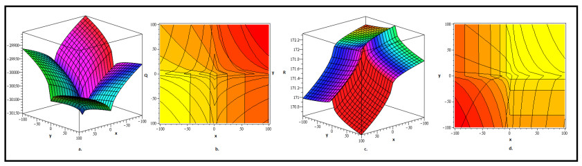
In this research work, we use the generalized Bernoulli equation method (gBEM) to investigate the chaotic nature of solitons in complex structured conformable coupled Maccari system (CCMS) which is a fractional generalization of a nonlinear model coupled Maccari system (CMS) initially created to simulate hydraulic systems. This key model has numerous applications in several disciplines such as hydrodynamics, optics, quantum mechanics and plasma physics. The proposed gBEM converts the CCMS into a set of nonlinear ordinary differential equations (NODEs) to construct fresh plethora of soliton solutions in the form of rational, trigonometric, hyperbolic, and exponential functions. To comprehend the dynamics of acquired solitons in CCMS, a series of 3D and counter plots are used which graphically illustrate and reveal two types of chaotic perturbations, namely axial and periodic perturbations in the acquired solitons. Furthermore, the efficiency and adaptability of our method in handling a range of nonlinear models in mathematical science and engineering are confirmed by our computational work.

References

[1]	A. A. Kilbas, H. M. Srivastava, J. J. Trujillo, Theory and applications of fractional differential equations, Elsevier, 2006.
[2]	H. Sun, Y. Zhang, D. Baleanu, W. Chen, Y. Chen, A new collection of real world applications of fractional calculus in science and engineering, Commun. Nonlinear Sci. Numer. Simul., 64 (2018), 213–231. https://doi.org/10.1016/j.cnsns.2018.04.019 doi: 10.1016/j.cnsns.2018.04.019
[3]	L. Debnath, Recent applications of fractional calculus to science and engineering, Int. J. Math. Math. Sci., 2003 (2003), 3413–3442.
[4]	O. Abu Arqub, Numerical simulation of time-fractional partial differential equations arising in fluid flows via reproducing Kernel method, Int. J. Numer. Methods Heat Fluid Flow, 30 (2020), 4711–4733.
[5]	E. M. Elsayed, K. Nonlaopon, The Analysis of the Fractional-Order Navier-Stokes Equations by a Novel Approach, J. Function Spaces, 2022 (2022), 8979447.
[6]	M. M. Al-Sawalha, A. Khan, O. Y. Ababneh, T. Botmart, Fractional view analysis of Kersten-Krasil'shchik coupled KdV-mKdV systems with non-singular kernel derivatives, AIMS Mathematics, 7 (2022), 18334–18359. http://doi.org/2010.3934/math.20221010
[7]	M. Alqhtani, K. M. Saad, W. M. Hamanah, Discovering novel soliton solutions for (3+ 1)-modified fractional Zakharov-Kuznetsov equation in electrical engineering through an analytical approach, Opt. Quantum Electron., 55 (2023), 1149.
[8]	B. K. Singh, P. Kumar, Fractional variational iteration method for solving fractional partial differential equations with proportional delay, Int. J. Differ. Eq., 2017 (2017), 5206380.
[9]	S. S. Ray, R. K. Bera, Analytical solution of a fractional diffusion equation by Adomian decomposition method, Appl. Math. Comput., 174 (2006), 329–336.
[10]	A. Elsaid, S. Shamseldeen, S. Madkour, Analytical approximate solution of fractional wave equation by the optimal homotopy analysis method, Eur. J. Pure Appl. Math., 10 (2017), 586–601.
[11]	J. Chen, F. Liu, V. Anh, Analytical solution for the time-fractional telegraph equation by the method of separating variables, J. Math. Anal. Appl., 338 (2008), 1364–1377.
[12]	Y. Nikolova, L. Boyadjiev, Integral transforms method to solve a time-space fractional diffusion equation, Fractional Calculus Appl. Anal., 13 (2010), 57–68.
[13]	M. A. Akinlar A, Secer, A. Cevikel Efficient solutions of system of fractional partial differential equations by the differential transform method, Adv. Differ. Equ., 2012 (2012), 188. http://doi.org/10.1186/1687-1847-2012-188 doi: 10.1186/1687-1847-2012-188
[14]	Y. Tian, J. Liu, A modified exp-function method for fractional partial differential equations, Therm. Sci., 25 (2021), 1237–1241.
[15]	S. J. Chen, Y. H. Yin, X. La, Elastic collision between one lump wave and multiple stripe waves of nonlinear evolution equations, Commun. Nonlinear Sci. Numer. Simul., 130 (2023), 107205. https://doi.org/10.1016/j.cnsns.2023.107205 doi: 10.1016/j.cnsns.2023.107205
[16]	O. Tasbozan, Y. Çenesiz, A. Kurt, New solutions for conformable fractional Boussinesq and combined KdV-mKdV equations using Jacobi elliptic function expansion method, Eur. Phys. J.Plus, 131 (2016), 244. https://doi.org/10.1140/epjp/i2016-16244-x doi: 10.1140/epjp/i2016-16244-x
[17]	X. La, S. J. Chen, Interaction solutions to nonlinear partial differential equations via Hirota bilinear forms: one-lump-multi-stripe and one-lump-multi-soliton types, Nonlinear Dyn., 103 (2021), 947–977.
[18]	Y. H. Yin, X. La, W. X. Ma, Backlund transformation, exact solutions and diverse interaction phenomena to a (3+ 1)-dimensional nonlinear evolution equation, Nonlinear Dyn., 108 (2022), 4181–4194.
[19]	D. Gao, X. La, M. S. Peng, Study on the (2+ 1)-dimensional extension of Hietarinta equation: soliton solutions and Bäcklund transformation, Phys. Scr., 98 (2023), 095225.
[20]	B. K. Singh, Fractional reduced differential transform method for numerical computation of a system of linear and nonlinear fractional partial differential equations, Int. J. Open Probl. Comput. Sci. Math., 238 (2016), 20–38.
[21]	S. T. Mohyud-Din, U. Khan, N. Ahmed, Khater method for nonlinear Sharma Tasso-Olever (STO) equation of fractional order, Results Phys., 7 (2017), 4440–4450.
[22]	A. A. Alderremy, N. Iqbal, S. Aly, K. Nonlaopon, Fractional series solution construction for nonlinear fractional reaction-diffusion Brusselator model utilizing Laplace residual power series, Symmetry, 14 (2022), 1944.
[23]	S. Phoosree, O. Suphattanakul, E. Maliwan, M. Senmoh, W. Thadee, Novel Solutions to Fractional Nonlinear Equations for Crystal Dislocation and Ocean Shelf Internal Waves via the Generalized Bernoulli Equation Method, Math. Modell. Eng. Probl., 10 (2023), 821. http://doi.org/10.18280/mmep.100312 doi: 10.18280/mmep.100312
[24]	O. T. Kolebaje, O. O. Popoola, Exact solution of fractional STO and Jimbo-Miwa equations with the generalized Bernoulli equation method, Afr. Rev. Phys., 9 (2014).
[25]	H. M. Baskonus, T. A. Sulaiman, H. Bulut, On the novel wave behaviors to the coupled nonlinear CMS with complex structure, Optik, 131 (2017), 1036–1043.
[26]	S. T. Demiray, Y. Pandir, H. Bulut, New solitary wave solutions of Maccari system, Ocean Eng., 103 (2015), 153–159.
[27]	J. Ahmad, S. Rani, N. B. Turki, N. A. Shah, Novel resonant multi-soliton solutions of time fractional coupled nonlinear Schrödinger equation in optical fiber via an analytical method, Results Phys., 52 (2023), 106761.
[28]	A. Maccari, The Maccari system as model system for rogue waves, Phys. Lett. A, 384 (2020), 126740.
[29]	U. N. Katugampola, New approach to a generalized fractional integral, Appl. Math. Comput., 218 (2011), 860–865. https://doi.org/10.1016/j.amc.2011.03.062 doi: 10.1016/j.amc.2011.03.062
[30]	S. G. Samko, A. A. Kilbas, O. I. Marichev, Fractional Integrals and Derivatives, In: Theory and Applications, Yverdon: Gordon and Breach, 1993.
[31]	V. E. Tarasov, On chain rule for fractional derivatives, Commun. Nonlinear Sci. Numer. Simul., 30 (2016), 1–4. https://doi.org/10.1016/j.cnsns.2015.06.007 doi: 10.1016/j.cnsns.2015.06.007
[32]	J. H. He, S. K. Elagan, Z. B. Li, Geometrical explanation of the fractional complex transform and derivative chain rule for fractional calculus, Phys. Lett. A, 376 (2012), 257–259.
[33]	M. Z. Sarikaya, H. Budak, H. Usta, On generalized the conformable fractional calculus, TWMS J. Appl. Eng. Math., 9 (2019), 792–799.
[34]	T. Abdeljawad, On conformable fractional calculus, J. Comput. Appl. Math. 279 (2015), 57–66.
[35]	R. Khalil, horani M. Al A. Yousef and M. Sababheh, A new definition of fractional derivative, J. Comput. Apll. Math., 264 (2014), 65–70.

Reader Comments

Your name:*

Email:*
© 2025 the Author(s), licensee AIMS Press. This is an open access article distributed under the terms of the Creative Commons Attribution License (http://creativecommons.org/licenses/by/4.0)