Skin dose enhancement from the application of skin-care creams using FF and FFF photon beams in radiotherapy: A Monte Carlo phantom evaluation

Megha Sharma ¹,
James C. L. Chow ^{2,3
,
,}

1.
Department of Physics, Ryerson University, Toronto, ON, M5B 2K3 Canada
2.
Radiation Medicine Program, Princess Margaret Cancer Centre, University Health Network, Toronto, ON, M5G 1X6 Canada
3.
Department of Radiation Oncology, University of Toronto, Toronto, ON, M5T 1P5 Canada

Received: 03 March 2020 Accepted: 21 April 2020 Published: 21 April 2020

Abstract
Full Text(HTML)

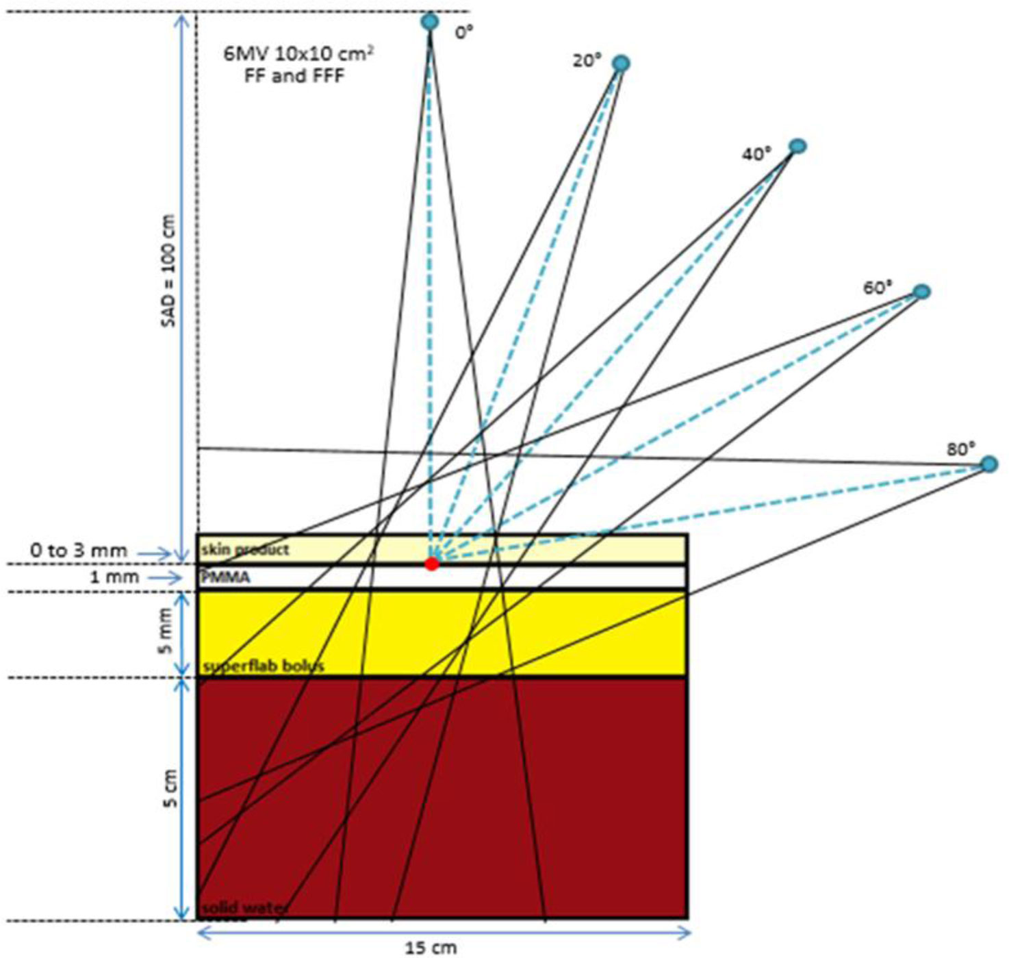
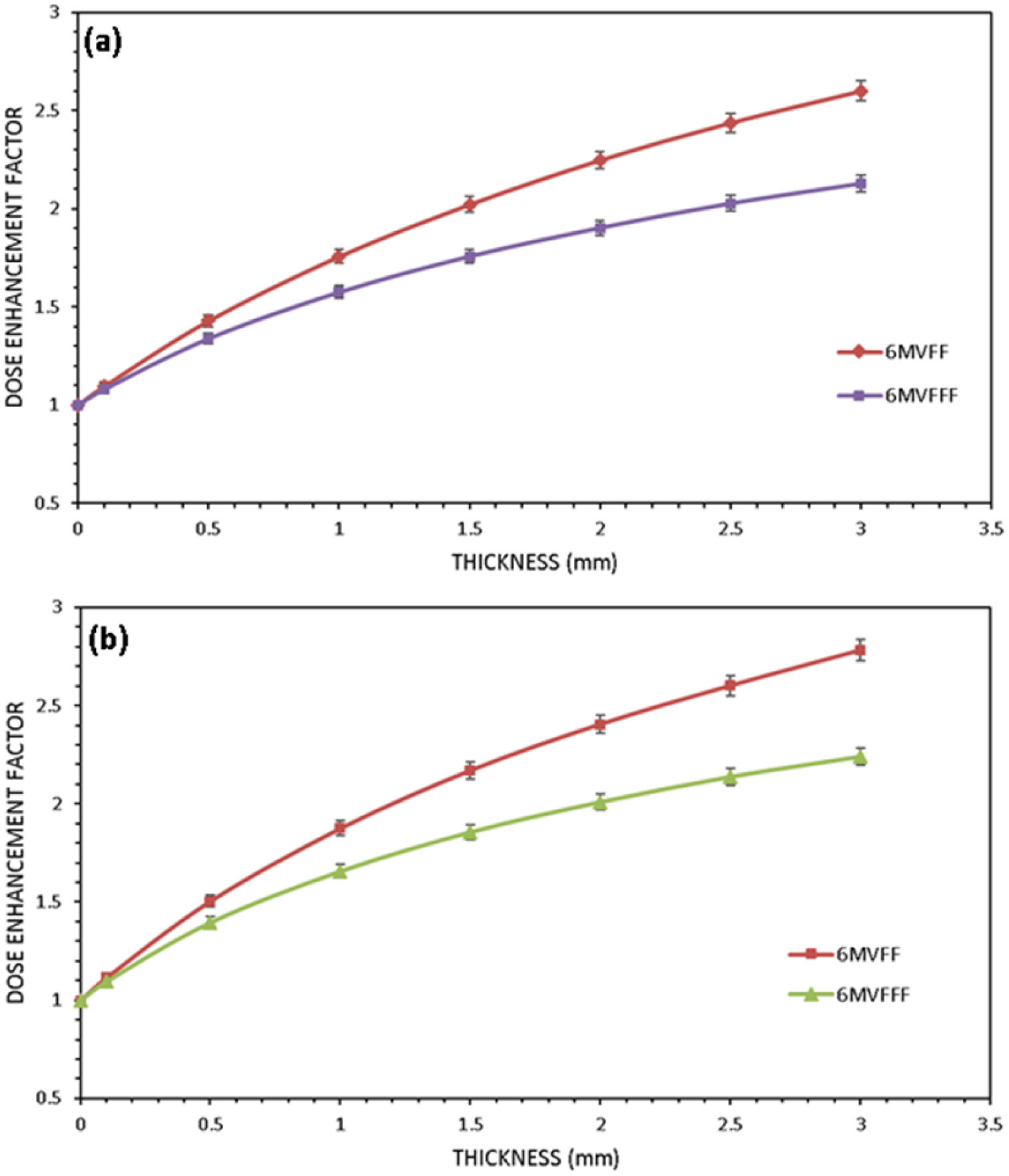
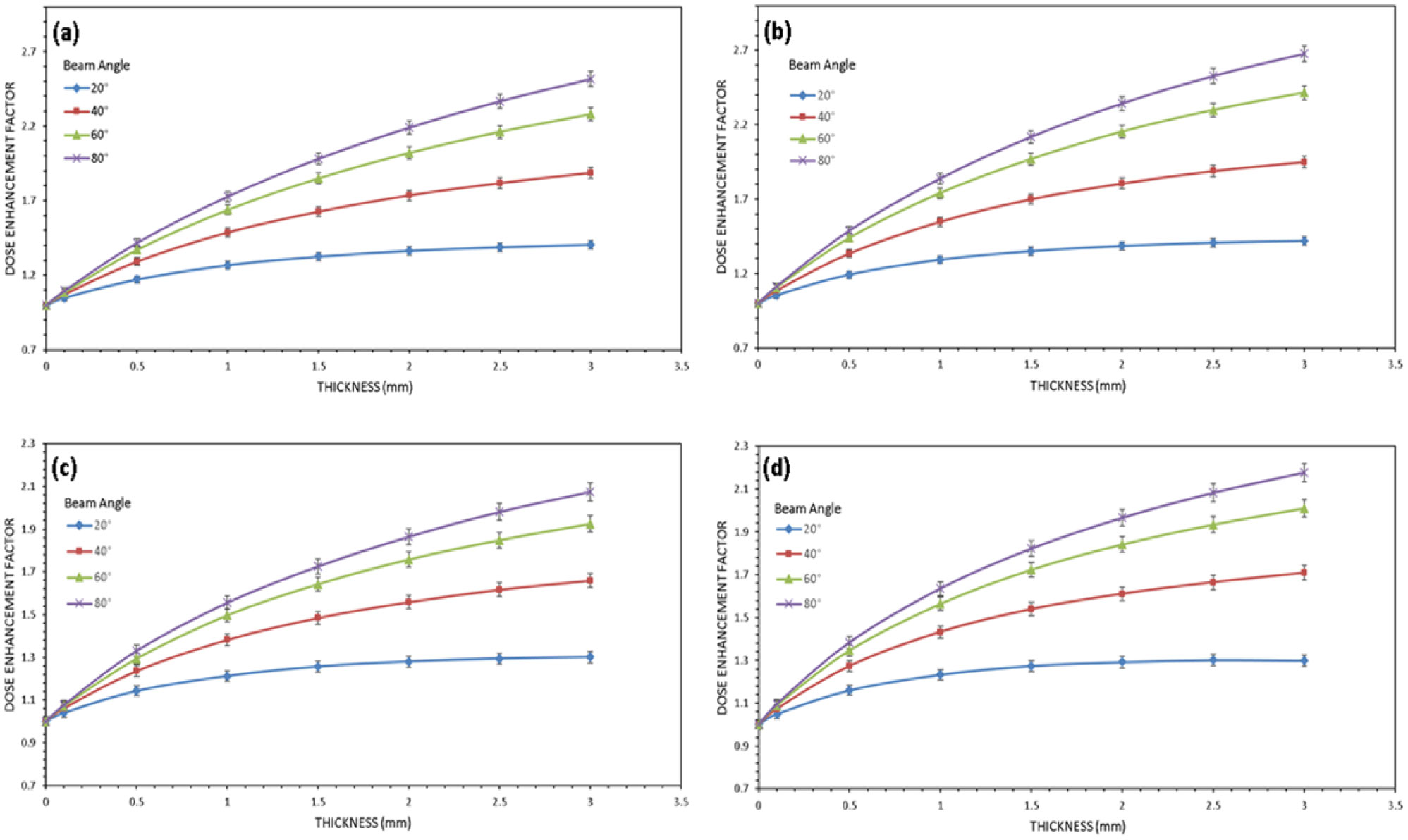
Skin-care cream is commonly applied to relieve skin redness in radiotherapy. However, using cream on the patient under the photon field would increase the skin dose in delivery. The aim of this study is to evaluate the dependences of skin dose enhancement on different beam and cream variables using Monte Carlo simulation. Using a solid water phantom with water-equivalent bolus, PMMA layer and cream layer, we irradiated it by 6 MV photon beams. Skin doses were calculated by varying the beam quality (flattening-filter (FF) and flattening-filter-free (FFF)), beam angle (0°–80°), skin-care cream type (water-based and silicon-based) and cream thickness (0–3 mm) using the EGSnrc Monte Carlo code. The densities of the water- and silicon-based cream were 0.92 and 1.14 g/cm³. The dose enhancement factor (DEF) defined as the ratio of the skin dose with skin-care cream to the skin dose without cream was calculated. It is found that the FF photon beam had higher DEF value than the FFF. For the water-based cream of 3 mm, the DEF for the FF beam was about 22.1% higher than that of the FFF. While for the silicon-based cream with the same thickness, the DEF was 24.2% higher. DEF value also increased with the beam angle. The DEF values were from 1.4 to 2.52 (water-based cream) and 1.42 to 2.68 (silicon-based cream) when the beam angle was increased from 20° to 80° using the 6 MV FF beams. Similarly, for the 6 MV FFF beams, the DEF values increased from 1.29 to 2.07 and 1.30 to 2.18 for the water- and silicon-based cream. These simulation results showed that the skin dose enhancement increased with an increase of beam angle, cream thickness, cream density, and the irradiation of FFF photon beams.
- skin-care cream,
- skin redness,
- skin dose,
- flattening-filter-free photon beam,
- Monte Carlo simulation
Citation: Megha Sharma, James C. L. Chow. Skin dose enhancement from the application of skin-care creams using FF and FFF photon beams in radiotherapy: A Monte Carlo phantom evaluation[J]. AIMS Bioengineering, 2020, 7(2): 82-90. doi: 10.3934/bioeng.2020008

Related Papers:

Abstract

Skin-care cream is commonly applied to relieve skin redness in radiotherapy. However, using cream on the patient under the photon field would increase the skin dose in delivery. The aim of this study is to evaluate the dependences of skin dose enhancement on different beam and cream variables using Monte Carlo simulation. Using a solid water phantom with water-equivalent bolus, PMMA layer and cream layer, we irradiated it by 6 MV photon beams. Skin doses were calculated by varying the beam quality (flattening-filter (FF) and flattening-filter-free (FFF)), beam angle (0°–80°), skin-care cream type (water-based and silicon-based) and cream thickness (0–3 mm) using the EGSnrc Monte Carlo code. The densities of the water- and silicon-based cream were 0.92 and 1.14 g/cm³. The dose enhancement factor (DEF) defined as the ratio of the skin dose with skin-care cream to the skin dose without cream was calculated. It is found that the FF photon beam had higher DEF value than the FFF. For the water-based cream of 3 mm, the DEF for the FF beam was about 22.1% higher than that of the FFF. While for the silicon-based cream with the same thickness, the DEF was 24.2% higher. DEF value also increased with the beam angle. The DEF values were from 1.4 to 2.52 (water-based cream) and 1.42 to 2.68 (silicon-based cream) when the beam angle was increased from 20° to 80° using the 6 MV FF beams. Similarly, for the 6 MV FFF beams, the DEF values increased from 1.29 to 2.07 and 1.30 to 2.18 for the water- and silicon-based cream. These simulation results showed that the skin dose enhancement increased with an increase of beam angle, cream thickness, cream density, and the irradiation of FFF photon beams.

Acknowledgment

The authors would like to thank Amir Owrangi of UT Southwestern Medical Centre for assistance in the phase-space files and photon energy spectra of the FF and FFF photon beams used in the Monte Carlo simulations.

Conflict of interest

The authors have no potential conflict of interest on financial or commercial matters associated with this study.

References

[1]	Delaney G, Jacob S, Featherstone C, et al. (2005) The role of radiotherapy in cancer treatment: estimating optimal utilization from a review of evidence-based clinical guidelines. Cancer 104: 1129-1137. doi: 10.1002/cncr.21324
[2]	Naylor W, Mallett J (2001) Management of acute radiotherapy induced skin reactions: a literature review. Eur J Oncol Nurs 5: 221-233. doi: 10.1054/ejon.2001.0145
[3]	Baumann BC, Verginadis II, Zeng C, et al. (2018) Assessing the validity of clinician advice that patients avoid use of topical agents before daily radiotherapy treatments. JAMA Oncol 4: 1742-1748. doi: 10.1001/jamaoncol.2018.4292
[4]	Harris R, Probst H, Beardmore C, et al. (2012) Radiotherapy skin care: A survey of practice in the UK. Radiography 18: 21-27. doi: 10.1016/j.radi.2011.10.040
[5]	Morley L, Cashell A, Sperduti A, et al. (2014) Evaluating the relevance of dosimetric considerations to patient teaching regarding skin care during radiation therapy. J Radiother Pract 13: 294-301. doi: 10.1017/S1460396913000241
[6]	Tse K, Morley L, Cashell A, et al. (2016) Dosimetric impacts on skin toxicity for patients using topical agents and dressings radiotherapy. J Radiother in Pract 15: 314-321. doi: 10.1017/S1460396916000285
[7]	Hadley SW, Kelly R, Lam K (2005) Effects of immobilization mask material on surface dose. J Appl Clin Med Phys 6: 1-7. doi: 10.1120/jacmp.v6i1.1957
[8]	Khan Y, Villarreal-Barajas JE, Udowicz M, et al. (2013) Clinical and dosimetric implications of air gaps between bolus and skin surface during radiation therapy. J Cancer Ther 4: 1251-1255. doi: 10.4236/jct.2013.47147
[9]	Løkkevik E, Skovlund E, Reitan JB, et al. (1996) Skin treatment with bepanthen cream versus no cream during radiotherapy: a randomized controlled trial. Acta Oncol 35: 1021-1026. doi: 10.3109/02841869609100721
[10]	Chow JCL, Grigorov GN (2008) Surface dosimetry for oblique tangential photon beams: A Monte Carlo simulation study. Med Phys 35: 70-76. doi: 10.1118/1.2818956
[11]	Chow JCL, Grigorov GN, Barnett RB (2006) Study on surface dose generated in prostate intensity-modulated radiation therapy treatment. Med Dosim 31: 249-258. doi: 10.1016/j.meddos.2005.07.002
[12]	Chow JCL, Owrangi AM (2016) A surface energy spectral study on the bone heterogeneity and beam obliquity using the flattened and unflattened photon beams. Rep Pract Oncol Radiother 21: 63-70. doi: 10.1016/j.rpor.2015.11.001
[13]	Chow JCL, Owrangi AM (2014) Dosimetric dependences of bone heterogeneity and beam angle on the unflattened and flattened photon beams: A Monte Carlo comparison. Radiat Phys Chem 101: 46-52. doi: 10.1016/j.radphyschem.2014.03.041
[14]	Bortfeld T (2006) IMRT: a review and preview. Phys Med Biol 51: R363. doi: 10.1088/0031-9155/51/13/R21
[15]	Jia J, Hui L, Chow JCL (2015) A leaf sequencing algorithm for multileaf collimator in intensity modulated radiotherapy. Rep Radiother Oncol 2: e4922.
[16]	Chow JCL, Grigorov GN, Yazdani N (2006) SWIMRT: A graphical user interface using sliding window algorithm to construct a fluence map machine file. J Appl Clin Med Phys 7: 69-85. doi: 10.1120/jacmp.v7i2.2231
[17]	Sharma SD (2011) Unflattened photon beams from the standard flattening filter free accelerators for radiotherapy: advantages, limitations and challenges. J Med Phys 36: 123-125. doi: 10.4103/0971-6203.83464
[18]	Chow JCL, Owrangi AM (2019) Mucosal dosimetry on unflattened photon beams: A Monte Carlo phantom study. Biomed Phys Eng Express 5: 015007. doi: 10.1088/2057-1976/aaeaaa
[19]	Chow JCL, Jiang R, Leung MKK (2011) Dosimetry of oblique tangential photon beams calculated by superposition/convolution algorithms: a Monte Carlo evaluation. J Appl Clin Med Phys 12: 108-121. doi: 10.1120/jacmp.v12i1.3424
[20]	Chow JCL (2018) Recent progress in Monte Carlo simulation of gold nanoparticle radiosensitization. AIMS Biophys 5: 231-244. doi: 10.3934/biophy.2018.4.231
[21]	Rogers DWO (2006) Fifty years of Monte Carlo simulations for medical physics. Phys Med Biol 51: R287. doi: 10.1088/0031-9155/51/13/R17
[22]	Kawrakow I, Mainegra-Hing E, Rogers DWO, et al. (2000) The EGSnrc code system: Monte Carlo simulation of electron and photon transport. NRCC Report PIRS-701 Ottawa: NRC, Available from: https://nrc-cnrc.github.io/EGSnrc/doc/pirs701-egsnrc.pdf.
[23]	Walters B, Kawrakow I, Rogers DWO (2005) DOSXYZnrc users manual. NRCC Report PIRS-794revB Ottawa: NRC, Available from: https://nrc-cnrc.github.io/EGSnrc/doc/pirs794-dosxyznrc.pdf.
[24]	Constantin M, Perl J, LoSasso T, et al. (2011) Modeling the TrueBeam linac using a CAD to Geant4 geometry implementation: dose and IAEA-compliant phase space calculations. Med Phys 38: 4018-4024. doi: 10.1118/1.3598439
[25]	Sardari D, Maleki R, Samavat H, et al. (2010) Measurement of depth-dose of linear accelerator and simulation by use of GEANT4 computer code. Rep Pract Oncol Radiother 15: 64-68. doi: 10.1016/j.rpor.2010.03.001

Reader Comments

your name:*

Email:*
© 2020 the Author(s), licensee AIMS Press. This is an open access article distributed under the terms of the Creative Commons Attribution License (http://creativecommons.org/licenses/by/4.0)