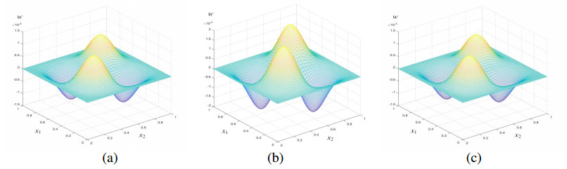
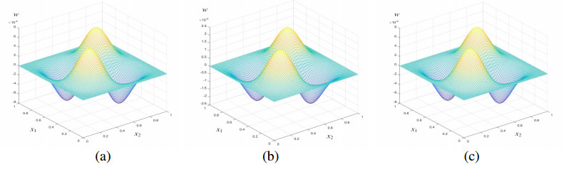
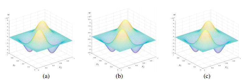
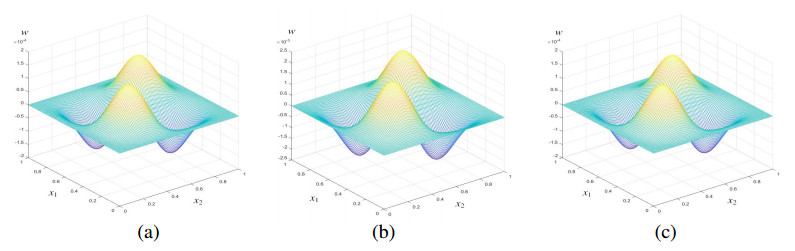
The main purpose of this paper was to study the reduced-dimension of unknown classical two-grid finite element (CTGFE) solution coefficient vectors for the nonlinear time-fractional wave (NTFW) equation by using proper orthogonal decomposition (POD). For this purpose, a CTGFE method with unconditional stability for the NTFW equation and the error estimates of CTGFE solutions were reviewed. Then, the CTGFE method was rewritten into matrix form, and the unknown solution coefficient vectors in the matrix CTGFE method were reduced by the POD method, so a new reduced-dimension TGFE (RDTGFE) method was created. The biggest contribution of this paper consists in analyzing theoretically the existence, stability, and errors of the RDTGFE solutions, and in applications, verifying the correctness of the obtained theoretical results and the advantages of the RDTGFE method. The RDTGFE method can not only greatly reduce the unknowns of the CTGFE method and the simplify computational process but also greatly save CPU runtime and improve the computational efficiency. Therefore, the RDTGFE method is worth studying and spreading.
Citation: Liang He, Yihui Sun, Zhenglong Chen, Fei Teng, Chao Shen, Zhendong Luo. The POD-based reduced-dimension study on the two-grid finite element method for the nonlinear time-fractional wave equation[J]. AIMS Mathematics, 2025, 10(2): 3408-3427. doi: 10.3934/math.2025158
The main purpose of this paper was to study the reduced-dimension of unknown classical two-grid finite element (CTGFE) solution coefficient vectors for the nonlinear time-fractional wave (NTFW) equation by using proper orthogonal decomposition (POD). For this purpose, a CTGFE method with unconditional stability for the NTFW equation and the error estimates of CTGFE solutions were reviewed. Then, the CTGFE method was rewritten into matrix form, and the unknown solution coefficient vectors in the matrix CTGFE method were reduced by the POD method, so a new reduced-dimension TGFE (RDTGFE) method was created. The biggest contribution of this paper consists in analyzing theoretically the existence, stability, and errors of the RDTGFE solutions, and in applications, verifying the correctness of the obtained theoretical results and the advantages of the RDTGFE method. The RDTGFE method can not only greatly reduce the unknowns of the CTGFE method and the simplify computational process but also greatly save CPU runtime and improve the computational efficiency. Therefore, the RDTGFE method is worth studying and spreading.

| [1] | C. Cattani, H. M. Srivastava, X. J. Yang, Fractional dynamics, Berlin: Emerging Science Publishers, 2015. |
| [2] | R. Hilfer, Applications of fractional calculus in physics, Singapore: World Scientific, 2000. |
| [3] | R. L. Magin, Fractional calculus in bioengineering, Danbury: Begell House Publishers, 2006. |
| [4] |
H. Ding, A high-order numerical algorithm for two-dimensional time-space tempered fractional diffusion-wave equation, Appl. Numer. Math., 135 (2019), 30–46. https://doi.org/10.1016/j.apnum.2018.08.005 doi: 10.1016/j.apnum.2018.08.005

|
| [5] |
R. Du, Y. Yan, Z. Liang, A high-order scheme to approximate the Caputo fractional derivative and its application to solve the fractional diffusion wave equation, J. Comput. Phys., 376 (2019), 1312–1330. https://doi.org/10.1016/j.jcp.2018.10.011 doi: 10.1016/j.jcp.2018.10.011
|
| [6] |
Z. Xing, L. Wen, Numerical analysis and fast implementation of a fourth-order difference scheme for two-dimensional space-fractional diffusion equations, Appl. Math. Comput., 346 (2019), 155–166. https://doi.org/10.1016/j.amc.2018.10.057 doi: 10.1016/j.amc.2018.10.057
|
| [7] |
Z. Luo, H. Wang, A highly efficient reduced-order extrapolated finite difference algorithm for time-space tempered fractional diffusion-wave equation, Appl. Math. Lett., 102 (2020), 106090. https://doi.org/10.1016/j.aml.2019.106090 doi: 10.1016/j.aml.2019.106090
|
| [8] |
Y. Zhou, Z. Luo, An optimized Crank-Nicolson finite difference extrapolating model for the fractional-order parabolic-type sine-Gordon equations, Adv. Differ. Equ., 2019 (2019), 1. https://doi.org/10.1186/s13662-018-1939-6 doi: 10.1186/s13662-018-1939-6
|
| [9] |
C. Çelik, M. Duman, Finite element method for a symmetric tempered fractional diffusion equation, Appl. Numer. Math., 120 (2017), 270–286. https://doi.org/10.1016/j.apnum.2017.05.012 doi: 10.1016/j.apnum.2017.05.012
|
| [10] |
J. Lin, J. Bai, S. Reutskiy, J. Lu, A novel RBF-based meshless method for solving time-fractional transport equations in 2D and 3D arbitrary domains, Eng. Comput., 39 (2023), 1905–1922. https://doi.org/10.1007/s00366-022-01601-0 doi: 10.1007/s00366-022-01601-0
|
| [11] |
K. Li, Z. Tan, A two-grid fully discrete Galerkin finite element approximation for fully nonlinear time-fractional wave equations, Nonlinear Dyn., 111 (2023), 8497–8521. https://doi.org/10.1007/s11071-023-08265-5 doi: 10.1007/s11071-023-08265-5
|
| [12] |
J. Xu, A novel two-grid method for semilinear elliptic equations, SIAM J. Sci. Comput., 15 (1994), 231–237. https://doi.org/10.1137/0915016 doi: 10.1137/0915016
|
| [13] |
D. Shi, Q. Liu, An efficient nonconforming finite element two-grid method for Allen-Cahn equation, Appl. Numer. Math., 98 (2019), 374–380. https://doi.org/10.1016/j.aml.2019.06.037 doi: 10.1016/j.aml.2019.06.037
|
| [14] |
D. Shi, R. Wang, Unconditional superconvergence analysis of a two-grid finite element method for nonlinear wave equations, Appl. Numer. Math., 150 (2020), 38–50. https://doi.org/10.1016/j.apnum.2019.09.012 doi: 10.1016/j.apnum.2019.09.012
|
| [15] |
Y. Liu, Y. Du, H. Li, J. Li, S. He, A two-grid mixed finite element method for a nonlinear fourth-order reaction-diffusion problem with time-fractional derivative, Comput. Math. Appl., 70 (2015), 2474–2492. https://doi.org/10.1016/j.camwa.2015.09.012 doi: 10.1016/j.camwa.2015.09.012
|
| [16] | Z. Luo, Finite element and reduced dimension methods for partial differential equations, Beijing: Springer and Science Press of China, 2024. |
| [17] |
F. Teng, Z. Luo, A natural boundary element reduced-dimension model for uniform high-voltage transmission line problem in an unbounded outer domain, Comput. Appl. Math., 43 (2024), 106. https://doi.org/10.1007/s40314-024-02617-6 doi: 10.1007/s40314-024-02617-6
|
| [18] | Z. Luo, G. Chen, Proper orthogonal decomposition methods for partial differential equations, London: Academic Press of Elsevier, 2019. |
| [19] |
H. Li, Z. Song, A reduced-order finite element method based on proper orthogonal decomposition for the Allen-Cahn model, J. Math. Anal. Appl., 500 (2021), 125103. https://doi.org/10.1016/j.jmaa.2021.125103 doi: 10.1016/j.jmaa.2021.125103
|
| [20] |
A. K. Alekseev, D. A. Bistrian, A. E. Bondarev, I. M. Navon, On linear and nonlinear aspects of dynamic mode decomposition, Int. J. Numer. Meth. Fluids, 82 (2016), 348–371. https://doi.org/10.1002/fld.4221 doi: 10.1002/fld.4221
|
| [21] |
J. Du, I. M. Navon, J. Zhu, F. Fang, A. K. Alekseev, Reduced order modeling based on POD of a parabolized Navier-Stokes equations model Ⅱ: Trust region POD 4D VAR data assimilation, Comput. Math. Appl., 65 (2013), 380–394. https://doi.org/10.1016/j.camwa.2012.06.001 doi: 10.1016/j.camwa.2012.06.001
|
| [22] |
K. Li, T. Huang, L. Li, S. Lanteri, L. Xu, B. Li, A reduced-order discontinuous Galerkin method based on POD for electromagnetic simulation, IEEE Trans. Antennas Propag., 66 (2018), 242–254. https://doi.org/10.1109/TAP.2017.2768562 doi: 10.1109/TAP.2017.2768562
|
| [23] |
Y. Li, H. Li, Y. Zeng, Z. Luo, A preserving accuracy two-grid reduced-dimensional Crank-Nicolson mixed finite element method for nonlinear wave equation, Appl. Numer. Math., 202 (2024), 1–20. https://doi.org/10.1016/j.apnum.2024.04.010 doi: 10.1016/j.apnum.2024.04.010
|
| [24] |
L. Jing, F. Teng, M. Feng, H. Li, J. Yang, Z. Luo, A novel dimension reduction model based on POD and two-grid Crank-Nicolson mixed finite element methods for 3D nonlinear elastodynamic sin-Gordon problem, Commun. Nonlinear Sci. Numer. Simul., 140 (2025), 108409. https://doi.org/10.1016/j.cnsns.2024.108409 doi: 10.1016/j.cnsns.2024.108409
|
| [25] |
X. Hou, Y. Li, Q. Deng, Z. Luo, A novel dimensionality reduction iterative method for the unknown coefficient vectors in TGFECN solutions of unsaturated soil water flow problem, J. Math. Anal. Appl., 543 (2025), 128930. https://doi.org/10.1016/j.jmaa.2024.128930 doi: 10.1016/j.jmaa.2024.128930
|
| [26] |
Y. Li, F. Teng, Y. Zeng, Z. Luo, Two-grid dimension reduction method of Crank-Nicolson mixed finite element solution coefficient vectors for the fourth-order extended Fisher-Kolmogorov equation, J. Math. Anal. Appl., 538 (2024), 128168. https://doi.org/10.1016/j.jmaa.2024.128168 doi: 10.1016/j.jmaa.2024.128168
|
| [27] |
H. Li, Y. Li, Y. Zeng, Z. Luo, A reduced-dimension extrapolation two-grid Crank-Nicolson finite element method of unknown solution coefficient vectors for spatial fractional nonlinear Allen-Cahn equations, Comput. Math. Appl., 167 (2024), 110–122. https://doi.org/10.1016/j.camwa.2024.05.007 doi: 10.1016/j.camwa.2024.05.007
|
| [28] |
H. Li, R. Yang, Analysis of two spectral Galerkin approximation schemes for solving the perturbed FitzHugh-Nagumo neuron model, Comput. Math. Appl., 143 (2023), 1–9. https://doi.org/10.1016/j.camwa.2023.04.033 doi: 10.1016/j.camwa.2023.04.033
|
| [29] |
Z. Song, D. Li, D. Wang, H. Li, A modified Crank Nicolson finite difference method preserving maximum-principle for the phase-field model, J. Math. Anal. Appl., 526 (2023), 127271. https://doi.org/10.1016/j.jmaa.2023.127271 doi: 10.1016/j.jmaa.2023.127271
|
| [30] | G. Zhang, Y. Lin, Notes on functional analysis, in Chinese, Beijing: Peking University Press, 2011. |
Figures(6) / Tables(1)

Liang He, Yihui Sun, Zhenglong Chen, Fei Teng, Chao Shen, Zhendong Luo. The POD-based reduced-dimension study on the two-grid finite element method for the nonlinear time-fractional wave equation[J]. AIMS Mathematics, 2025, 10(2): 3408-3427. doi: 10.3934/math.2025158


 DownLoad: