


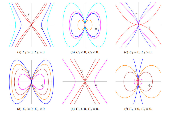
Figure 1.
The phase portraits of (4.2) for C1C2≥0.
This study systematically investigates the dynamics of the perturbed Schrödinger-Hirota equation with cubic-quintic-septic nonlinearity under spatiotemporal dispersion, providing insights into soliton propagation in dispersive media. We begin by examining the system's phase portrait and chaotic behavior, followed by the derivation of exact traveling wave solutions, including optical solitons and periodic solutions, using an enhanced algebraic method. The findings are vividly illustrated through three-dimensional and two-dimensional graphical simulations, which analyze the impact of key parameters on the solutions. This study not only presents a variety of optical soliton solutions, but also clarifies the underlying dynamics, offering theoretical guidance for fiber optic communication systems and holding significant applied value for achieving more efficient and reliable optical communications.
Citation: Tianyong Han, Ying Liang, Wenjie Fan. Dynamics and soliton solutions of the perturbed Schrödinger-Hirota equation with cubic-quintic-septic nonlinearity in dispersive media[J]. AIMS Mathematics, 2025, 10(1): 754-776. doi: 10.3934/math.2025035
| [1] | Elsayed M. E. Zayed, Mona El-Shater, Khaled A. E. Alurrfi, Ahmed H. Arnous, Nehad Ali Shah, Jae Dong Chung . Dispersive optical soliton solutions with the concatenation model incorporating quintic order dispersion using three distinct schemes. AIMS Mathematics, 2024, 9(4): 8961-8980. doi: 10.3934/math.2024437 |
| [2] | Abeer S. Khalifa, Hamdy M. Ahmed, Niveen M. Badra, Wafaa B. Rabie, Farah M. Al-Askar, Wael W. Mohammed . New soliton wave structure and modulation instability analysis for nonlinear Schrödinger equation with cubic, quintic, septic, and nonic nonlinearities. AIMS Mathematics, 2024, 9(9): 26166-26181. doi: 10.3934/math.20241278 |
| [3] | Noha M. Kamel, Hamdy M. Ahmed, Wafaa B. Rabie . Solitons unveilings and modulation instability analysis for sixth-order coupled nonlinear Schrödinger equations in fiber bragg gratings. AIMS Mathematics, 2025, 10(3): 6952-6980. doi: 10.3934/math.2025318 |
| [4] | Dumitru Baleanu, Kamyar Hosseini, Soheil Salahshour, Khadijeh Sadri, Mohammad Mirzazadeh, Choonkil Park, Ali Ahmadian . The (2+1)-dimensional hyperbolic nonlinear Schrödinger equation and its optical solitons. AIMS Mathematics, 2021, 6(9): 9568-9581. doi: 10.3934/math.2021556 |
| [5] | Ninghe Yang . Exact wave patterns and chaotic dynamical behaviors of the extended (3+1)-dimensional NLSE. AIMS Mathematics, 2024, 9(11): 31274-31294. doi: 10.3934/math.20241508 |
| [6] | Islam Samir, Hamdy M. Ahmed, Wafaa Rabie, W. Abbas, Ola Mostafa . Construction optical solitons of generalized nonlinear Schrödinger equation with quintuple power-law nonlinearity using Exp-function, projective Riccati, and new generalized methods. AIMS Mathematics, 2025, 10(2): 3392-3407. doi: 10.3934/math.2025157 |
| [7] | Mahmoud Soliman, Hamdy M. Ahmed, Niveen Badra, M. Elsaid Ramadan, Islam Samir, Soliman Alkhatib . Influence of the β-fractional derivative on optical soliton solutions of the pure-quartic nonlinear Schrödinger equation with weak nonlocality. AIMS Mathematics, 2025, 10(3): 7489-7508. doi: 10.3934/math.2025344 |
| [8] | A. K. M. Kazi Sazzad Hossain, M. Ali Akbar . Solitary wave solutions of few nonlinear evolution equations. AIMS Mathematics, 2020, 5(2): 1199-1215. doi: 10.3934/math.2020083 |
| [9] | Da Shi, Zhao Li, Dan Chen . New traveling wave solutions, phase portrait and chaotic patterns for the dispersive concatenation model with spatio-temporal dispersion having multiplicative white noise. AIMS Mathematics, 2024, 9(9): 25732-25751. doi: 10.3934/math.20241257 |
| [10] | Nafissa Toureche Trouba, Mohamed E. M. Alngar, Reham M. A. Shohib, Haitham A. Mahmoud, Yakup Yildirim, Huiying Xu, Xinzhong Zhu . Novel solitary wave solutions of the (3+1)–dimensional nonlinear Schrödinger equation with generalized Kudryashov self–phase modulation. AIMS Mathematics, 2025, 10(2): 4374-4411. doi: 10.3934/math.2025202 |
This study systematically investigates the dynamics of the perturbed Schrödinger-Hirota equation with cubic-quintic-septic nonlinearity under spatiotemporal dispersion, providing insights into soliton propagation in dispersive media. We begin by examining the system's phase portrait and chaotic behavior, followed by the derivation of exact traveling wave solutions, including optical solitons and periodic solutions, using an enhanced algebraic method. The findings are vividly illustrated through three-dimensional and two-dimensional graphical simulations, which analyze the impact of key parameters on the solutions. This study not only presents a variety of optical soliton solutions, but also clarifies the underlying dynamics, offering theoretical guidance for fiber optic communication systems and holding significant applied value for achieving more efficient and reliable optical communications.
The application of nonlinear partial differential equations (NPDEs) in the field of optics originated with the emergence of nonlinear fiber optics, where the nonlinear Schrödinger equation (NLSE) serves as a key model for describing the evolution of optical pulses in fibers. This equation was introduced by Erwin Schrödinger in 1927. With the advancement of technology, the NLSE has transcended its foundational role in quantum mechanics and has become a crucial model in the field of optics, particularly in the realm of optical fiber communications. Since the seminal work by Hasegawa and Tappert in 1973, the NLSE has been extensively studied, revealing the fascinating world of optical solitons [1]. These solitary waves, capable of maintaining their shape over long distances, have become the backbone of modern optical communication due to their potential for high-speed and high-capacity data transmission. The NLSE serves as a fundamental framework for understanding the dynamics of light pulses and soliton propagation in dispersive media, with applications spanning from information transmission to the development of optical switches and ultra-short pulse lasers [2,3].
Various mathematical models have been developed based on the nonlinear Schrödinger equation for applications in nonlinear optics, plasma, ion-acoustic waves, and other fields. These models include the Radhakrishnan-Kundu-Lakshmanan equation [4] which introduces additional nonlinear terms to study nonlinear wave phenomena; the Chen-Lee-Liu equation for describing nonlinear soliton behavior in optics[5]; the Lakshmanan-Porsezian-Daniel equation for investigating soliton behavior in nonlinear optics [6]; the Fokas-Lenells equation for nonlinear wave phenomena [7]; the Schrödinger-Hirota equation (SHE) for soliton behavior in nonlinear optics [8]; the Zabolotskaya-Khokhlov model [9] for sound and ultrasound; the Biswas-Milovic equation with more complex nonlinear terms for studying wave phenomena [10]; the Maxwell-Bloch equation for atomic interactions and photon behavior [11]; the Manakov model for nonlinear optical signal propagation in fibers [12]; the Sasa-Satsuma equation for nonlinear wave phenomena in plasma [13]; the Rangwala-Rao equation for nonlinear optics in specific scenarios [14]; the Gerdjikov-Ivanov equation for quantum propagation, nonlinear optics, and weakly nonlinear water wave phenomena [15]; the Hirota-Maccari system for studying nonlinear wave phenomena [16], as well as other models.
The SHE, for instance, is a notable derivative obtained through Lie transformation, offering unique insights into the behavior of optical pulses in dispersive optical fibers. The incorporation of varying self-phase modulation terms, such as cubic-quintic-septic laws, has further enriched our comprehension of soliton dynamics. Constructing various soliton solutions of the NLSE not only helps to explain the physical characteristics of light signals propagating in nonlinear media, but also contributes to the updating or development of mathematical models. Therefore, an increasing number of scholars are dedicated to developing effective analytical and numerical procedures to generate various optical soliton solutions. These include the the enhanced Kudryashov's scheme [17], F-expansion technique [18], complete discriminant system [19,20], the extended trial function method [21], Sardar sub-equation procedure [22], planar dynamic system method [23], tanh function method [24,25,26], extended tanh function method [27,28], and more. These methodologies have been instrumental in deciphering the physical properties of soliton solutions and providing a theoretical underpinning for soliton transmission in fiber optics.
The perturbed SHE, a particular variant of the NLSE that incorporates higher-order nonlinear effects, has garnered attention for its ability to provide a more nuanced description of soliton propagation in dispersive media. The SHE is an extension of the NLSE, incorporating higher-order nonlinear terms to capture more complex dynamics. This evolution is a testament to the continuous endeavor to model the intricate behavior of light in optical fibers. In 2004, Wazwaz made a significant stride by introducing a third-order dispersion term into the NLSE, leading to an equation of the form [29]
| iQt+12Qxx+|Q|2Q+iλQxxx=0. | (1.1) |
This formulation marked a pivotal moment in the construction of optical solitons, providing a more nuanced understanding of their propagation characteristics. Some authors have also introduced third-order nonlinear terms into NLSE [30]. As researchers delved deeper into the study of weakly nonlinear, dispersive, and hyperbolic systems in the context of nonlinear fiber optics, the SHE emerged as a crucial model [31]. The equation
| iQt+12Qxx+|Q|2Q+iλ(Qxxx+6|U|2Qx)=0 | (1.2) |
was proposed to encapsulate the essence of wave propagation in these systems, offering a more comprehensive framework for analysis and modeling. In many fields of science and technology, such as adaptive optical systems, tunable optical filters, and optical communication systems, there is often a requirement for dispersive devices to be time-dependent, leading to the need for systems with spatiotemporal dispersion. As a result, the spatiotemporal dispersive model SHE [32], given by
| iQt+aQxx+bQxt+c1|Q|2U+i(λQxxx+d1|Q|2Qx)=0 | (1.3) |
introduced a new dimension to the study, accounting for the effects of both space and time on wave propagation. Some authors have studied the wave propagation of SHE with Kerr or power law nonlinearity [33,34,35], some have constructed optical solitons with both spatiotemporal dispersion SHE [36,37,38], and some researchers have studied the dynamic behavior of random SHE with noise [39,40].
Furthermore, scenarios such as ultrafast optics, strong field effects in nonlinear media, photonic integrated circuits, and extreme physical conditions often lead to the presence of higher-order nonlinearities in signal propagation. In order to study the propagation laws of waves under more general conditions, various higher-order nonlinearity terms have been introduced into SHE, also known as the perturbed Schrödinger-Hilliotta equation (PSHE). Researchers have employed a variety of effective methods to address SHE equations with different nonlinear terms. For instance, the extended auxiliary equation method has been applied to PSHE with cubic-quintic-septic law nonlinearity [41], the Kudryashov scheme to PHSE with anti-cubic law in the presence of spatiotemporal dispersion [42], the Hirota bilinear method to PSHE with quadratic-cubic nonlinearity and inter-model dispersion [43], the (1/G′)-expansion method to those with cubic-quintic nonlinearity [44], modified auxiliary equation method [45,46], complete discriminant system to SHE with Kerr law nonlinearity [47,48,49], modified simple equation integration approach to PSHE with spatio-temporal dispersion and Kerr law nonlinear [50,51], and so forth [52,53].
Despite extensive research, there remain gaps in our understanding of the perturbed SHE, particularly in the context of chaotic behavior and optical solitons. Future work should aim to bridge these gaps, exploring the interplay between higher-order nonlinearities, dispersion, and the dynamics of solitons. Additionally, the impact of external perturbations on the stability and propagation of solitons remains an area ripe for investigation.
However, the complexity of real optical systems, characterized by spatiotemporal dispersion, self-phase modulation, and other higher-order effects, poses significant challenges for deriving exact solutions from the Schrödinger equation. These optical systems, which simultaneously contain spatiotemporal dispersion and high-order nonlinear terms, are capable of adapting to more complex environments, yet have received relatively little theoretical research attention. While there is a significant amount of work in this field, typically relying on approximations or numerical simulations, it is still necessary to fully capture the rich dynamics of solitons in optical fibers. Building on this motivation, this has motivated our exploration of the PSHE with cubic-quintic-septic law incorporating spatiotemporal dispersion. The governing model, given by [53] as
| iQt+αQxx+βQxt+(λ1|Q|2+λ2|Q|4+λ3|Q|6)Q+i(η1Qxxx+η2|Q|2Qx)=i(μ1Qx+μ2(|Q|2Q)x+μ3(|Q|2)xQ), | (1.4) |
serves as the focal point of our investigation, where Q(x,t) represents the complex soliton profile, and the coefficients α, β, η1, and η2 capture the effects of group velocity dispersion, and spatiotemporal dispersion, and λ1, λ2, and λ3 are the nonlinearities of varying orders, respectively. The coefficients of μ1, μ2 and μ3 are the inter-modal dispersion, self-steepening, and the nonlinear dispersions. Equation (1.4) contains higher-order nonlinear terms and serves as a generalization of other nonlinear SHE. When λ3=0,μ1=μ2=μ3=0, Eq (1.4) reduces to the dispersive SHE [41].
By revisiting the evolution and research history of the SHE, this study identifies the gaps and limitations in the current understanding of the model, particularly concerning the higher-order nonlinearity and dispersion effects. Although several authors have employed the previously mentioned methods to study the PSHE, the types and quantities of solutions constructed remain limited. Recent literature, including references [42,53], reports the construction of only a very few exact solutions, which is insufficient for a comprehensive understanding of the equation. To further advance our research, we will employ an enhanced algebraic method. The findings of this research are expected to contribute to the theoretical framework of soliton dynamics and offer insights for the practical design of advanced fiber optic communication systems.
This manuscript is meticulously organized to present our findings in a coherent and methodical manner. The structure of this paper is as follows: Section 2 initiates with a pertinent transformation of the focal model, simplifying the complex nonlinear ordinary differential equation derived from our analysis. Section 3 delves into the characteristics of the phase portrait, employing the theory of planar dynamical systems, to elucidate the chaotic behavior inherent in the perturbed system. Section 4 harnesses the integration theory of dynamical systems to meticulously construct exact traveling wave solutions, which encapsulate a spectrum of optical solitons and periodic solutions. The penultimate sections amalgamate our findings with existing literature, engaging in a comprehensive discussion and summarization of the results, and charting a course for future research endeavors. The concluding section synthesizes the principal findings, underscores their implications for nonlinear optics and fiber optic communication systems, and suggests directions for subsequent scholarly pursuits.
Let the traveling wave transformation ϕ(x,t)=ϕ(ξ),ξ=kx+ωt reduce the nonlinear partial differential equation
| N(ϕ,ϕt,ϕx,ϕxx,⋯)=0 | (2.1) |
to a nonlinear ordinary differential equation:
| Q(ϕ,ϕ′,ϕ″,⋯)=0. | (2.2) |
Step 1: Assume that Eq (2.2) has a solution of the form:
| ϕ=n∑i=−naiui, | (2.3) |
satisfying the constraint:
| u′2=4∑i=0τiui. | (2.4) |
where u=u(ξ), ai,τj,i=−n,−n+1,⋯,n,j=0,⋯,4, τ4≠0, are constants to be determined. With the assistance of the software MAPLE, the solution of Eq (2.4) can be obtained as shown below:
Set 1:
| u1(ξ)=√−τ2τ4sech[√τ2(ξ−ξ0)],τ0=τ1=τ3=0,τ2>0,τ4<0, | (2.5) |
| u2(ξ)=√τ2τ4csch[√τ2(ξ−ξ0)],τ0=τ1=τ3=0,τ2>0,τ4>0, | (2.6) |
where ξ0 is the constant of integration.
Set 2:
| u3(ξ)=√−τ22τ4tanh[√−τ22(ξ−ξ0)],τ0=τ224τ4,τ1=τ3=0,τ2<0,τ4>0, | (2.7) |
| u4(ξ)=√−τ22τ4coth[√−τ22(ξ−ξ0)],τ0=τ224τ4,τ1=τ3=0,τ2<0,τ4>0. | (2.8) |
Set 3: τ1=τ3=0,σ=τ0τ4τ22,τ4>0,
| u5(ξ)=±√τ22τ4√1+m2+m√8+m24cs(√τ2√2√1+m2+m√8+m24(ξ−ξ0),m),τ2>0,0<σ<14,m=√2√1−4σ√1+√1−σ. | (2.9) |
| u6(ξ)=√τ2τ4√1−m22m2−1cn(√τ22m2−1(ξ−ξ0),m),τ2>0,σ<0,m=√√1−4σ+1√2√1−4σ.u7(ξ)=asn(√τ4p(ξ−ξ0),m)+bcn(√τ4p(ξ−ξ0),m)csn(√τ4p(ξ−ξ0),m)+dcn(√τ4p(ξ−ξ0),m),σ>14,τ2>0, | (2.10) |
where a=−s√l2+s2, b=√l2+s2(l+√l2+s2), c=s, d=l+√l2+s2s, l=√2√σ|τ2τ4|−τ2τ4, s=12√2√σ|τ2τ4|+τ2τ4, p=−√l2+s2(l√l2+s2+l2+s2)s3√(l2+s2)(2(l2+s2)32l+6√l2+s2l3+2l√l2+s2s2+8l4+8l2s2+s4), m2=4l√l2+s2(2l2+s2+2l√l2+s2)s4+8l2(l2+s2)+4l(2l2+s2)√l2+s2.
Set 4: τ1=τ3=0,τ4<0,
| u8(ξ)=√τ2|τ4|m2dn(√τ2m2(ξ−ξ0),m),τ2>0,0<σ<14,m=√2√1−4σ+1, | (2.11) |
| u9(ξ)=√m22m2−1τ22τ4cn(√τ222m2−1(ξ−ξ0),m),τ2>0,σ<0,m=√√1−4σ+1√2√1−4σ, | (2.12) |
| u10(ξ)=√τ2τ4m21−2m2cn(√1−2m2√−τ2(ξ−ξ0),m),τ2<0,σ<0,m=√√1−4σ−1√2√1−4σ. | (2.13) |
Set 5: τ1=τ3=0,
| u11(ξ)=3℘′(ξ−ξ0;g2,g3)√τ4(6℘(ξ−ξ0;g2,g3)+τ2),τ4>0, | (2.14) |
| u12(ξ)=√τ0(6℘(ξ−ξ0;g2,g3)+τ2)3℘′(ξ−ξ0;g2,g3),τ0>0, | (2.15) |
where ℘(ξ−ξ0;g2,g3) is the Weierstrass elliptic function.
Set 6: τ0=τ1=0,τ2>0
| u13(ξ)=−τ2sech2[12√τ2(ξ−ξ0)]±2√τ2τ4tanh[12√τ2(ξ−ξ0)]+τ3,τ4>0, | (2.16) |
| u14(ξ)=τ2csch2[12√τ2(ξ−ξ0)]±2√τ2τ4coth[12√τ2(ξ−ξ0)]+τ3,τ4>0, | (2.17) |
| u15(ξ)=−τ2τ3sech2[√τ22(ξ−ξ0)]τ23−τ2τ4(1−tanh[√τ22(ξ−ξ0)])2,τ3≠0, | (2.18) |
| u16(ξ)=τ2τ3csch2[√τ22(ξ−ξ0)]τ23−τ2τ4(1−coth[√22(ξ−ξ0)])2,τ3≠0. | (2.19) |
Step 2: Determine n according to the balance principle, such that the highest derivative term and the highest power term in Eq (2.2) have equal degrees.
Step 3: Substitute Eqs (2.3) and (2.4) together into Eq (2.2) to obtain the coefficients ai,τj,i=−n,−n+1,⋯,n,j=0,⋯,4.
Step 4: Combining the conclusions from Step 1 to Step 3, the solution to Eq (2.1) can be derived based on Eq (2.3) and the solutions of Eq (2.4).
To solve Eq (1.4), we can utilize the following transformation:
| Q(x,t)=P(ξ)ei(−κx+ωt+φ0),ξ=x−vt, | (3.1) |
where κ is the wave number, ω is the angular frequency, φ0 is phase constant, and v is the velocity. Substituting transformation (3.1) into Eq (1.4) and separating the real and imaginary parts yields
| η1P′′′−((3μ2+2μ3−η2)P2+(2α−βv)κ+3κ2η1−βω+v+μ1)P′=0, | (3.2) |
| (α−βv+3η1κ)P′′−(η1κ3+ακ2+(μ1−βω)κ+ω)P−((a−η2)κ−λ1)P3+λ2P5+λ3P7=0. | (3.3) |
If Eq (3.2) is integrated and the integration constant is assumed as zero, then we obtain
| 3η1P′′+(η2−3μ2−2μ3)P3+3(−3η1κ2+(βv−2α)κ+βω−μ1−v)P=0. | (3.4) |
Equation (3.4) gives the following constraints:
| η1=0,η2=3μ2+2μ3,ν=2ακ−βω+μ1βκ−1. | (3.5) |
The balance of Eq (3.3) will give a fraction 13, so we will use the substitution
| P(ξ)=ϕ1/3(ξ), |
to induce a transformation in which Eq (3.3) is converted to
| 9(λ1+2κ(μ2+μ3))ϕ83+9λ2ϕ103+3(α−βv)ϕϕ′′+2(βv−α)(ϕ′)2+9λ3ϕ4+9(−ακ2+ω(βκ−1)−κμ1)ϕ2=0. | (3.6) |
For the integrability of Eq (3.6), we set
| λ1=−2κ(μ2+μ3),λ2=0. | (3.7) |
Then,
| ϕϕ′′=23(ϕ′)2+C1ϕ2+C2ϕ4, | (3.8) |
where C1=−3(βκ−1)(ακ2−ω(βκ−1)+κμ1)α(βκ+1)−β2ω+βμ1, C2=3λ3(βκ−1)α(βκ+1)−β2ω+βμ1.
To analyze the dynamical behavior of Eq (3.7) using the planar dynamical systems method [20,23], we convert it into the following two-dimensional system:
| {dϕdξ=y,dydξ=1ϕ(23y2+C1ϕ2+C2ϕ4). | (4.1) |
Let dξ=ϕdη. Then, system (4.1) has the equivalent topology structure to the following regular systems:
| {dϕdη=yϕ,dydη=23y2+C1ϕ2+C2ϕ4, | (4.2) |
except for the straight line ϕ=0.
Then, the first integration of system (4.2) is
| H(ϕ,y)=ϕ−43y2−3C1ϕ23−34C2ϕ83=h,h∈R. | (4.3) |
If C1C2≥0, then system (4.2) has a unique equilibrium point P0(0,0). If C1C2<0, then system (4.2) has three equilibrium points P0(0,0), P1(−√−C1C2,0), and P2(√−C1C2,0). Without loss of generality, let C21+C22≠0.
In order to study the dynamic behavior of system (4.2), the Jacobian matrix is introduced
| J(ϕ,y)=(yϕ2C1ϕ+4C2ϕ343y). | (4.4) |
According to the theory of planar dynamical systems, when the trace tr(J)<0, P is the saddle point, and when the determinant det(J)>0 and tr(J)=0, P is the center. Therefore, the equilibrium points can be classified by the parameters C1 and C2 as follows:
● If C1C2≥0, then system (4.2) has a unique degenerate equilibrium point P0.
● If C1>0 and C2<0, then system (4.2) has three equilibrium points, where P0 is the degenerate equilibrium point, and P1 and P2 are centers.
● If C1<0 and C2>0, then system (4.2) has three equilibrium points, where P0 is the degenerate equilibrium point, and P1 and P2 are saddle points.
We use the phase portraits to demonstrate the dynamic behavior of the system near the equilibrium point, as shown in Figures 1 and 2.

Following our comprehensive analysis of the phase portrait of the system (4.2), we now turn to the fascinating phenomenon of chaos that emerges when the system is subjected to periodic perturbations. The introduction of such perturbations can significantly alter the dynamics of the system, leading to behaviors that are not only complex, but also highly sensitive to initial conditions. The periodic perturbations of Eq (4.2) are shown below:
| {dϕdη=yϕ,dydη=23y2+C1ϕ2+C2ϕ4+f0cos(ωη), | (4.5) |
where f0 and ω represent the amplitude and frequency of the external force perturbation, respectively.
Our methodology commences with a numerical simulation of the perturbed system, meticulously tracking the trajectories of the system's state variables over time. This simulation serves as a foundation for identifying the onset of chaotic behavior, characterized by aperiodic and unpredictable trajectories that diverge exponentially from nearby initial states.
Subsequently, the phase space of the perturbed system is analyzed through a series of two-dimensional phase diagrams. These diagrams reveal the intricate interplay between periodic orbits and chaotic regions, offering a visual representation of the system's dynamical complexity.
The temporal evolution of the system is also scrutinized through time series analysis, which provides insights into the temporal patterns that govern the system's behavior. Significant differences in the time series resulting from different initial values are beneficial in identifying the chaotic behavior of the system.
Finally, the Poincaré section, a method involving the intersection of the phase space trajectory with a specific plane, offers a snapshot of the system's state at discrete intervals. This technique is invaluable for identifying periodic orbits, quasiperiodic motions, and the intricate structures that characterize chaotic attractors.
The sensitivity of the perturbed system (4.5) to initial conditions is a hallmark of chaotic dynamics. To elucidate this property, we present comparative simulations in Figures 3 and 4, showcasing the system's behavior under two distinct sets of parameters.


In Figure 3, the parameters are set to f0=2.05, ω=2.891, c1=0, and c2=−1. The 3D trajectory plot, 2D phase portraits, time series plot, and Poincaré section of Eq (4.5) are depicted, each illustrating the profound impact of initial conditions on the system's trajectory. The red solid line represents the system's evolution from the initial condition x0=0.05,y0=0.07, while the blue dashed line corresponds to x0=0.08,y0=0.10. The stark divergence between these trajectories, evident in the figure, underscores the system's inherent complexity and the unpredictable nature of its evolution.
Moving to Figure 4, the parameters remain consistent with those in Figure 3. Here, the red solid line traces the system's path originating from x0=14,y0=0, whereas the blue dashed line is initiated at x0=13,y0=0. Similar to the observations in Figure 3, even minute variations in initial conditions give rise to dramatically different trajectories, reinforcing the notion that the system's behavior is intricate and highly contingent on its starting point.
The juxtaposition of these figures not only highlights the system's sensitivity to initial conditions, but also serves as a testament to the rich and varied dynamical repertoire that emerges from the interplay of deterministic equations and periodic perturbations. Such visual evidence of chaos is instrumental in advancing our understanding of the system's behavior.
According to the homogeneous balance principle, it is known that n=1, thus Eq (2.2) can be expressed as:
| ϕ(ξ)=a1u(ξ)+a−1u(ξ)+a0. | (5.1) |
Substituting Eq (5.1), Eq (2.4) into (3.7), and setting the coefficients of the common powers of to zero, we solve the system to derive the solutions for Eq (1.4).
Ultimately, the solutions obtained are shown below:
Set 1: The bell shaped soliton solution and the singular soliton solution.
If τ0=τ1=τ3=0, τ2=3C1, a−1 =0,a0 =0,a1=±√43τ4C2, the respective solutions are
| Q1,1=±{2√−C1C2sech[√3C1(x−vt−ξ0)]}13ei(−κx+ωt+φ0),C1>0,C2<0, | (5.2) |
| Q1,2=±{2√C1C2csch[√3C1(x−vt−ξ0)]}13ei(−κx+ωt+φ0),C1>0,C2>0. | (5.3) |
Here and in the rest of this article, Qi,j=Qi,j(x,t).
Set 2: The combo dark-sigular soliton solution.
If τ0=τ224τ4,τ1=τ3=0, the corresponding solutions are
Result 1: a−1=±τ2√3C23τ4,a0=0,a1=∓√43C2τ4, τ2=−32C1, C1>0, C2>0.
| Q2,1=[±√C1C23coth(√−τ22(x−vt−ξ0))−√C1C2tanh(√34C1(kx+ωt−ξ0))]13×ei(−κx+ωt+φ0), | (5.4) |
| Q2,2=[±√C1C23tanh(√−τ22(x−vt−ξ0))−√C1C2coth(√34C1(x−vt−ξ0))]13×ei(−κx+ωt+φ0). | (5.5) |
Result 2: a0=±√−τ224C2,a1=0, τ2=127C1,C1<0,C2>0.
| Q2,3={a−1√−6C17τ4tanh[√−67C1(x−vt−ξ0)]±√−C114C2}13ei(−κx+ωt+φ0), | (5.6) |
| Q2,4={a−1√−6C17τ4coth[√−67C1(x−vt−ξ0)]±√−C114C2}13ei(−κx+ωt+φ0). | (5.7) |
Set 3: The Jacobi elliptic function solutions.
If τ1=τ3=0,σ=τ0τ4τ22,τ4>0, the respective solutions are
(1) a−1=±√τ02C2,a0=±√−C112C2,τ2=2C1,
| Q3,1={±2√τ0τ42C1C2√m2+m√8+m2+4sc(√C1√1+m2+m√8+m24(x−vt−ξ0),m)±√−C112C2}13×ei(−κx+ωt+φ0), | (5.8) |
where τ2>0, 0<σ<14, m=√2√1−4σ√1+√1−4σ, C1>0, C2<0.
(2) a−1=±√τ02C2,a0=±√−C112C2,a1=0,τ2=2C1,τ0<0,τ4>0.
| Q3,2(ξ)={±√τ0τ4(2m2−1)4C1C2(1−m2)cn(√2C12m2−1(x−vt−ξ0),m)±√−C112C2}13ei(−κx+ωt+φ0), | (5.9) |
where σ<0,C2<0,m=√√1−4σ+1√2√1−4σ.
(3) a−1=±√τ02C2,a0=0,a1=±√τ42C2,τ0>0,τ4>0.
| Q3,3(ξ)={±√τ02C21Φ±√τ42C2Φ}13ei(−κx+ωt+φ0),σ>14,τ2>0, | (5.10) |
where Φ=asn(√τ4p(x−vt−ξ0),m)+bcn(√τ4p(x−vt−ξ0),m)csn(√τ4p(x−vt−ξ0),m)+dsn(√τ4p(x−vt−ξ0),m), C2>0, a=−s√l2+s2, b=√l2+s2(l+√l2+s2), c=s, d=l+√l2+s2s, p=−√l2+s2(l√l2+s2+l2+s2)s3√(l2+s2)(2(l2+s2)32l+6√l2+s2l3+2l√l2+s2s2+8l4+8l2s2+s4), m2=4l√l2+s2(2l2+s2+2l√l2+s2)s4+8l2(l2+s2)+4l(2l2+s2)√l2+s2.
Set 4: The Jacobi elliptic function solutions.
If τ1=τ3=0,σ=τ0τ4τ22,τ4<0, the corresponding solutions are
(1) a−1=±√τ02C2,a0=0,a1=±√τ224C2,τ2>0,τ0<0,
| Q4,1={±√τ2224C2|τ4|m2dn(√τ2m2(x−vt−ξ0),m)±√τ0|τ4|2C2τ2m2dn(√τ2m2(x−vt−ξ0),m)}, | (5.11) |
where C2<0, 0<σ<14, m=√2√1−4k+1.
Set 5: Weierstrass elliptic function solution.
τ1=τ3=0.
Result 1: a−1=0,a0=√−τ224C2,a1=√τ42C2,τ2=127C1.
| Q5,1={√τ42C23℘′(x−vt−ξ0;g2,g3)6℘(x−vt−ξ0;g2,g3)+τ2+√−τ224C2}13ei(−κx+ωt+φ0),τ4>0,C2>0. | (5.12) |
Result 2: a−1=√4τ03C2,a0=0,a1=±√4τ43C2.
| Q5,2={√4τ0τ43C26℘(x−vt−ξ0;g2,g3)+τ23℘′(x−vt−ξ0;g2,g3)+√12C2℘′(x−vt−ξ0;g2,g3)6℘(x−vt−ξ0;g2,g3)+τ2}13ei(−κx+ωt+φ0), | (5.13) |
where τ0>0,C2>0.
Set 6: Hyperbolic solutions.
τ0=τ1=0.
Result 1: a0=τ32τ2a−1,a1=0,τ2=τ324τ4,τ3>0,C1=3τ324τ4,C2=0.
| Q6,1={±a−12√τ2τ4tanh(τ34√τ4(x−vt−ξ0))+τ3τ2sech2(τ34√τ4(x−vt−ξ0))+2τ4τ3a−1}13ei(−κx+ωt+φ0), | (5.14) |
| Q6,2={±a−12√τ2τ4coth(τ34√τ4(x−vt−ξ0))+τ3τ2csch2(τ34√τ4(x−vt−ξ0))+2τ4τ3a−1}13ei(−κx+ωt+φ0). | (5.15) |
The solutions Q6,1 and Q6,2 are unbounded function solutions.
Result 2: a−1=0,a0=±√−C1C2,a1=±√4τ43C2,τ2=−2C1, C1<0,C2>0.
| Q6,3={±√τ43C24C1sech2(√−2C12(x−vt−ξ0))2√−2C1τ4tanh(√−2C12(x−vt−ξ0))+τ3±√−C1C2}13ei(−κx+ωt+φ0). | (5.16) |
| Q6,4={±√τ43C24C1csch2(√−2C12(x−vt−ξ0))2√−2C1τ4coth(√−2C12(x−vt−ξ0))+τ3±√−C1C2}13ei(−κx+ωt+φ0). | (5.17) |
The solutions Q6,3 is the bright solution, and Q6,4 is the dark solutions respectively.
The graphical simulations of the soliton, kink soliton, and periodic solutions are presented to provide an intuitive understanding of their spatial and temporal evolution. The 3D and 2D plots illustrate the distinctive wave patterns and dynamic behaviors, showcasing the versatility of the solutions derived from the PSHE. Figures 5(a)–8(a) depict the three-dimensional shapes of modes Q1,1, Q2,3, Q3,2 and Q6,3 respectively. The two-dimensional waveforms of these solutions at t=0, 1, and 2 are shown in Figures 5(b)–8(b). To enhance the explanation of the solutions, the real parts of these solutions are also illustrated in Figures 5(c)–8(c). It is worth noting that the solutions obtained in this study are numerous, and the above four solutions are representative.


As a key feature, this study investigates the dynamic behavior and analytical solutions of PSHE with both the temporal dispersion coefficient β and the seventh-order nonlinear coefficient λ3.
Understanding the sensitivity of the obtained solutions to these parameters is crucial for comprehending the stability and adaptability of optical solitons under different environmental conditions. The influence of the dispersion coefficient β on Q1,1 and Q2,3 is shown in Figures 9(a) and 10(a), while the impact of the nonlinear coefficient λ3 on the real parts of Q1,1 and Q2,3 is illustrated in Figures 9(b) and 10(b). Analysis of Figures 9 and 10 reveals a clear relationship between the magnitude of |β| and the amplitude of the optical soliton, indicating that an increase in |β| results in a larger soliton amplitude. In contrast, the influence of the nonlinearity parameter λ3 shows a more complex behavior: As λ3 increases, the amplitude of the optical soliton also increases; conversely, a decrease in λ3 leads to a reduction in the soliton amplitude. These observations underscore the critical role of these parameters in nonlinear optics, providing valuable insights for guiding both practical applications and further research in the field.


Now, let us compare the conclusions obtained in this paper with those obtained in the comparable literature.
The Perturbed Schrödinger-Hirota Equation (PSHE) has garnered significant attention from scholars in the field of nonlinear dynamics and partial differential equations. In this paper, we juxtapose our latest findings with those presented here to underscore the innovative aspects of our research.
Recent literature, specifically reference [53], employed SAE method to derive an exact solution expressed in terms of exponential functions. Similarly, reference [42] utilized NKS approach to study SHE with cubic nonlinearity, yielding three exact solutions represented by exponential functions.
In contrast to these studies, our work employs a phase portrait analysis to elucidate the underlying chaotic behavior associated with the PSHE. Furthermore, we have adopted the Exp-function Method (EAM) to obtain a comprehensive set of 16 solutions, which are expressed using hyperbolic functions, Jacobi elliptic functions, and Weierstrass elliptic functions. This approach has yielded a more profound understanding of the PSHE, as evidenced by the diversity and quantity of solutions obtained. The richness of the solution types and the sheer number of solutions presented in this paper not only advance the current body of knowledge, but also provide a more nuanced perspective on the dynamics of the PSHE. Our findings contribute significantly to the existing literature by offering a broader spectrum of exact solutions, thereby enhancing our ability to analyze and predict the behavior of complex nonlinear systems described by the PSHE.
This study investigates a theoretical model capable of adapting to complex environments with both spatiotemporal dispersion and high-order nonlinearities. The conclusions drawn from this research hold promising implications for future developments in the field. The main findings of this study are poised to exert a positive impact on the realms of nonlinear optics and fiber optic communication systems. The bifurcation analysis and the diverse soliton solutions presented in this paper have deepened our comprehension of soliton dynamics within complex media. The sensitivity analysis and investigation of chaotic behavior have shed light on the stability of solitons under perturbations, a factor critical for the practical application of optical communication technologies. The future research directions outlined in this paper, which include exploring higher-order nonlinear effects and developing more sophisticated models to capture the intricate dynamics of light in optical fibers, are conducive to enhancing the design and optimization of fiber optic systems. These endeavors will not only advance our theoretical understanding but also contribute to the practical advancements in the field of fiber optics. By providing a comprehensive analysis and a spectrum of solutions, this study has laid a solid foundation for further research and development in nonlinear optics, paving the way for innovative applications in fiber optic communication systems. The insights gained from this work are expected to inspire continued exploration and innovation, ultimately leading to more efficient and robust optical communication technologies.
Tianyong Han: Conceptualization, formal analysis, writing-review & editing, critical review; Ying Liang: Review, graphic drawing; Wenjie Fan: Methodology. All authors have read and approved the final version of the manuscript for publication.
The authors declare they have not used Artificial Intelligence (AI) tools in the creation of this article.
This work was supported by Sichuan Science and Technology Program (No.2023NSFSC0078), Dazhou Key Laboratory of Multidimensional Data Perception and Intelligent Information Processing (DWSJ2305), Digital Tianfu Cultural Innovation Key Laboratory Open Fund Project (TFWH-2024-06).
The authors declare that they have no competing interests.
| [1] |
A. Hasegawa, F. Tappert, Transmission of stationary nonlinear optical pulses in dispersive dielectric fibers. I. Anomalous dispersion, Appl. Phys. Lett., 23 (1973), 171. https://doi.org/10.1063/1.1654847 doi: 10.1063/1.1654847

|
| [2] |
T. Han, Z. Li, X. Zhang, Bifurcation and new exact traveling wave solutions to time-space coupled fractional nonlinear Schrödinger equation, Phys. Lett. A, 395 (2021), 127217. https://doi.org/10.1016/j.physleta.2021.127217 doi: 10.1016/j.physleta.2021.127217
|
| [3] |
L. Tang, Bifurcations and dispersive optical solitons for the nonlinear Schrödinger-Hirota equation in DWDM networks, Optik, 262 (2022), 169276. https://doi.org/10.1016/j.ijleo.2022.169276 doi: 10.1016/j.ijleo.2022.169276
|
| [4] |
K. Zhang, X. He, Z. Li, Bifurcation analysis and classification of all single traveling wave solution in fiber Bragg gratings with Radhakrishnan-Kundu-Lakshmanan equation, AIMS Math., 7 (2022), 16733–16740. https://doi.org/10.3934/math.2022918 doi: 10.3934/math.2022918
|
| [5] |
Z. Li, Qualitative analysis and explicit solutions of perturbed Chen-Lee-Liu equation with refractive index, Results Phys., 60 (2024), 107626. https://doi.org/10.1016/j.rinp.2024.107626 doi: 10.1016/j.rinp.2024.107626
|
| [6] |
C. A. Sarmasik, M. Ekici, Multi wave, kink, breather, Peregrine-like rational and interaction solutions for the concatenation model, Opt. Quant. Electron., 56 (2024), 256. https://doi.org/10.1007/s11082-023-05799-1 doi: 10.1007/s11082-023-05799-1
|
| [7] |
Z. Li, J. Liu, X. Xie, New single traveling wave solution in birefringent fibers or crossing sea waves on the high seas for the coupled Fokas-Lenells system, J. Ocean Eng. Sci., 8 (2023), 590–594. https://doi.org/10.1016/j.joes.2022.05.017 doi: 10.1016/j.joes.2022.05.017
|
| [8] |
L. Tang, Bifurcation analysis and multiple solitons in birefringent fibers with coupled Schrödinger-Hirota equation, Chaos Soliton. Fract., 161 (2022), 112383. https://doi.org/10.1016/j.chaos.2022.112383 doi: 10.1016/j.chaos.2022.112383
|
| [9] |
T. Han, H. Rezazadeh, U. R. Mati, High-order solitary waves, fission, hybrid waves and interaction solutions in the nonlinear dissipative (2+1)-dimensional Zabolotskaya-Khokhlov model, Phys. Scripta, 99 (2024), 115212. https://doi.org/10.1088/1402-4896/ad7f04 doi: 10.1088/1402-4896/ad7f04
|
| [10] |
Z. Li, E. Hussain, Qualitative analysis and optical solitons for the (1+1)-dimensional Biswas-Milovic equation with parabolic law and nonlocal nonlinearity, Results Phys., 56 (2024), 107304. https://doi.org/10.1016/j.rinp.2023.107304 doi: 10.1016/j.rinp.2023.107304
|
| [11] |
L. An, Y. Chen, L. Ling, Inverse scattering transforms for the nonlocal Hirota-Maxwell-Bloch system, J. Phys. A-Math. Theor., 56 (2023), 115201. https://doi.org/10.1088/1751-8121/acbb45 doi: 10.1088/1751-8121/acbb45
|
| [12] |
T. Han, Z. Li, K. Shi, G. C. Wu, Bifurcation and traveling wave solutions of stochastic Manakov model with multiplicative white noise in birefringent fibers, Chaos Soliton. Fract., 163 (2022), 112548. https://doi.org/10.1016/j.chaos.2022.112548 doi: 10.1016/j.chaos.2022.112548
|
| [13] |
M. Sadaf, S. Arshed, G. Akram, H. Shadab, A. S. M. Alzaidi, Traveling wave dynamics of the generalized Sasa-Satsuma equation by two integrating schemes, Opt. Quant. Electron., 56 (2024), 209. https://doi.org/10.1007/s11082-024-06900-y doi: 10.1007/s11082-024-06900-y
|
| [14] |
C. Peng, Z. Li, New traveling wave solutions and dynamic behavior analysis of the nonlinear Rangwala-Rao model, Results Phys., 54 (2023), 107096. https://doi.org/10.1016/j.rinp.2023.107096 doi: 10.1016/j.rinp.2023.107096
|
| [15] |
C. Liu, Z. Li, The dynamical behavior analysis of the fractional perturbed Gerdjikov-Ivanov equation, Results Phys., 59 (2024), 107537. https://doi.org/10.1016/j.rinp.2024.107537 doi: 10.1016/j.rinp.2024.107537
|
| [16] |
T. Han, L. Zhao, Bifurcation, sensitivity analysis and exact traveling wave solutions for the stochastic fractional Hirota-Maccari system, Results Phys., 47 (2023), 106349. https://doi.org/10.1016/j.rinp.2023.106349 doi: 10.1016/j.rinp.2023.106349
|
| [17] |
A. H. Arnous, A. Biswas, A. H. Kara, Y. Yildirim, L. Moraru, S. Moldovanu, Dispersive optical solitons and conservation laws of Radhakrishnan-Kundu-Lakshmanan equation with dual-power law nonlinearity, Heliyon, 9 (2023), e14036. https://doi.org/10.1016/j.heliyon.2023.e14036 doi: 10.1016/j.heliyon.2023.e14036
|
| [18] | Y. Yildirim, A. Biswas, S. Khan, M. Belic, Embedded solitons with χ(2) and χ(3) nonlinear susceptibilities, Semicond. Phys. Quant., 24 (2021), 160–165. |
| [19] |
J. Wang, Z. Li, A dynamical analysis and new traveling wave solution of the fractional coupled Konopelchenko-Dubrovsky model, Fractal Fract., 8 (2024), 341. https://doi.org/10.3390/fractalfract8060341 doi: 10.3390/fractalfract8060341
|
| [20] |
T. Han, K. Zhang, Y. Jiang, H. Rezazadeh, Chaotic pattern and solitary solutions for the (2+1)-dimensional Beta-fractional double-chain DNA system, Fractal Fract., 8 (2024), 415. https://doi.org/10.3390/fractalfract8070415 doi: 10.3390/fractalfract8070415
|
| [21] |
M. Ekici, A. Sonmezoglu, Optical solitons with Biswas-Arshed equation by extended trial function method, Optik, 177 (2019), 13–20. https://doi.org/10.1016/j.ijleo.2018.09.134 doi: 10.1016/j.ijleo.2018.09.134
|
| [22] |
S. Irshad, M. Shakeel, A. Bibi, M. Sajjad, K. S. Nisar, A comparative study of nonlinear fractional Schrödinger equation in optics, Mod. Phys. Lett. B, 37 (2023), 2250219. https://doi.org/10.1142/S0217984922502190 doi: 10.1142/S0217984922502190
|
| [23] |
T. Han, Y. Jiang, Bifurcation, chaotic pattern and traveling wave solutions for the fractional Bogoyavlenskii equation with multiplicative noise, Phys. Scripta, 99 (2024), 035207. https://doi.org/10.1088/1402-4896/ad21ca doi: 10.1088/1402-4896/ad21ca
|
| [24] | E. H. M. Abdullah, H. M. Ahmed, A. A. S. Zaghrout, A. I. A. Bahnasy, W. B. Rabie, Unveiling optical solitons in twin-core couplers with Kerr law of nonlinear refractive index using improved modified extended tanh function method, J. Optics, 2024. https://doi.org/10.1007/s12596-024-01971-2 |
| [25] |
W. B. Rabie, H. M. Ahmed, Diverse exact and solitary wave solutions to new extended KdV6 equation using IM extended tanh-function technique, Pramana-J. Phys., 98 (2024), 1–8. https://doi.org/10.1007/s12043-024-02767-6 doi: 10.1007/s12043-024-02767-6
|
| [26] |
M. S. Ghayad, N. M. Badra, H. M. Ahmed, W. B. Rabie, M. Mirzazadeh, M. S. Hashemi, Highly dispersive optical solitons in fiber Bragg gratings with cubic quadratic nonlinearity using improved modified extended tanh-function method, Opt. Quant. Electron., 56 (2024), 1184. https://doi.org/10.1007/s11082-024-07064-5 doi: 10.1007/s11082-024-07064-5
|
| [27] |
M. S. Ahmed, A. A. S. Zaghrout, H. M. Ahmed, I. Samir, Optical solitons for the stochastic perturbed Schrödinger-Hirota equation using two different methods, J. Opt., 53 (2024), 2631–2641. https://doi.org/10.1007/s12596-023-01403-7 doi: 10.1007/s12596-023-01403-7
|
| [28] |
O. El-Shamy, R. El-barkoki, H. M. Ahmed, W. Abbas, I. Samir, Extraction of solitons in multimode fiber for CHNLSEs using improved modified extended tanh function method, Alex. Eng. J., 106 (2024), 403–410. https://doi.org/10.1016/j.aej.2024.07.014 doi: 10.1016/j.aej.2024.07.014
|
| [29] |
A. Biswas, Stochastic perturbation of optical solitons in Schrödinger-Hirota equation, Opt. Commun., 239 (2004), 461–466. https://doi.org/10.1016/j.optcom.2004.06.047 doi: 10.1016/j.optcom.2004.06.047
|
| [30] |
Y. S. Ozkan, E. Yasar, A. R. Seadawy, On the multi-waves, interaction and Peregrine-like rational solutions of perturbed Radhakrishnan-Kundu-Lakshmanan equation, Phys. Scripta, 95 (2020), 085205. https://doi.org/10.1088/1402-4896/ab9af4 doi: 10.1088/1402-4896/ab9af4
|
| [31] |
X. Geng, Y. Lv, Darboux transformation for an integrable generalization of the nonlinear Schrödinger equation, Nonlinear Dyn., 69 (2012), 1621–1630. https://doi.org/10.1007/s11071-012-0373-7 doi: 10.1007/s11071-012-0373-7
|
| [32] |
S. Kumar, K. Singh, R. Gupta, Coupled Higgs field equation and Hamiltonian amplitude equation: Lie classical approach and (G′/G)-expansion method, Pramana, 79 (2012), 41–60. https://doi.org/10.1007/s12043-012-0284-7 doi: 10.1007/s12043-012-0284-7
|
| [33] |
W. J. Liu, L. H. Pang, P. Wong, M. Lei, Z. Y. Wei, Dynamic solitons for the perturbed derivative nonlinear Schrödinger equation in nonlinear optics, Laser Phys., 25 (2015), 065401. https://doi.org/10.1088/1054-660X/25/6/065401 doi: 10.1088/1054-660X/25/6/065401
|
| [34] |
M. Ekici, M. Mirzazadeh, A. Sonmezoglu, M. Z. Ullah, M. Asma, Q. Zhou, et al., Dispersive optical solitons with Schrödinger-Hirota equation by extended trial equation method, Optik, 136 (2017), 451–461. https://doi.org/10.1016/j.ijleo.2017.02.042 doi: 10.1016/j.ijleo.2017.02.042
|
| [35] | A. J. M. Jawad, S. Kumar, A. Biswas, Solition solutions of a few nonlinear wave equations in engineering sciences, Sci. Iran., 21 (2014), 861–869. |
| [36] | A. J. M. Jawad, A. Biswas, Y. Yildirim, A. A. Alghamdi, Dispersive optical solitons with Schrödinger-Hirota equation by a couple of integration schemes, J. Optoelectron. Adv. M., 25 (2023), 203–209. |
| [37] |
N. Ozdemir, A. Secer, M. Ozisik, M. Bayram, Perturbation of dispersive optical solitons with Schrödinger-Hirota equation with Kerr law and spatio-temporal dispersion, Optik, 265 (2022), 169545. https://doi.org/10.1016/j.ijleo.2022.169545 doi: 10.1016/j.ijleo.2022.169545
|
| [38] |
M. Inc, A. I. Aliyu, A. Yusuf, D. Baleanu, Dispersive optical solitons and modulation instability analysis of Schrödinger-Hirota equation with spatio-temporal dispersion and Kerr law nonlinearity, Superlattice, Superlattice. Microst., 113 (2018), 319–327. https://doi.org/10.1016/j.spmi.2017.11.010 doi: 10.1016/j.spmi.2017.11.010
|
| [39] |
C. Peng, L. Tang, Z. Li, D. Chen, Qualitative analysis of stochastic Schrödinger-Hirota equation in birefringent fibers with spatiotemporal dispersion and parabolic law nonlinearity, Results Phys., 51 (2023), 106729. https://doi.org/10.1016/j.rinp.2023.106729 doi: 10.1016/j.rinp.2023.106729
|
| [40] |
E. M. E. Zayed, R. M. A. Shohib, M. E. M. Alngar, Dispersive optical solitons in magneto-optic waveguides with stochastic generalized Schrödinger-Hirota equation having multiplicative white noise, Optik, 271 (2022), 170069. https://doi.org/10.1016/j.ijleo.2022.170069 doi: 10.1016/j.ijleo.2022.170069
|
| [41] |
N. Ozdemir, S. Altun, A. Secer, M. Ozisik, M. Bayram, Optical solitons for the dispersive Schrödinger-Hirota equation in the presence of spatio-temporal dispersion with parabolic law, Eur. Phys. J. Plus, 139 (2023), 551. https://doi.org/10.1140/epjp/s13360-023-04196-7 doi: 10.1140/epjp/s13360-023-04196-7
|
| [42] |
S. A. Durmus, N. Ozdemir, A. Secer, M. Ozisik, M. Bayram, Examination of optical soliton solutions for the perturbed Schrödinger-Hirota equation with anti-cubic law in the presence of spatiotemporal dispersion, Eur. Phys. J. Plus, 139 (2024), 464. https://doi.org/10.1140/epjp/s13360-024-05272-2 doi: 10.1140/epjp/s13360-024-05272-2
|
| [43] |
S. T. R. Rizvi, A. R. R. Seadawy, N. Farah, S. Ahmed, Transformation and interactions among solitons in metamaterials with quadratic-cubic nonlinearity and inter-model dispersion, Int. J. Mod. Phys. B, 37 (2023), 2350087. https://doi.org/10.1142/S021797922350087X doi: 10.1142/S021797922350087X
|
| [44] |
A. Yokus, H. M. Baskonus, Dynamics of traveling wave solutions arising in fiber optic communication of some nonlinear models, Soft Comput., 26 (2022), 13605–13614. https://doi.org/10.1007/s00500-022-07320-4 doi: 10.1007/s00500-022-07320-4
|
| [45] |
M. Inc, A. I. Aliyu, A. Yusuf, D. Baleanu, Optical and singular solitary waves to the PNLSE with third order dispersion in Kerr media via two integration approaches, Optik, 163 (2018), 142–151. https://doi.org/10.1016/j.ijleo.2018.02.084 doi: 10.1016/j.ijleo.2018.02.084
|
| [46] |
A. Houwe, S. Abbagari, G. Betchewe, M. Inc, S. Y. Doka, K. T. Crepin, et al., Exact optical solitons of the perturbed nonlinear Schrödinger-Hirota equation with Kerr law nonlinearity in nonlinear fiber optics, Open Phys., 18 (2020), 526–534. https://doi.org/10.1515/phys-2020-0177 doi: 10.1515/phys-2020-0177
|
| [47] |
Y. Akbar, H. Alotaibi, A novel approach to explore optical solitary wave solution of the improved perturbed nonlinear Schrödinger equation, Opt. Quant. Electron., 54 (2022), 534. https://doi.org/10.1007/s11082-022-03922-2 doi: 10.1007/s11082-022-03922-2
|
| [48] |
T. Han, Z. Li, C. Li, Bifurcation analysis, stationary optical solitons and exact solutions for generalized nonlinear Schrödinger equation with nonlinear chromatic dispersion and quintuple power-law of refractive index in optical fibers, Physica A, 615 (2023), 128599. https://doi.org/10.1016/j.physa.2023.128599 doi: 10.1016/j.physa.2023.128599
|
| [49] |
L. Tang, Optical solitons perturbation and traveling wave solutions in magneto-optic waveguides with the generalized stochastic Schrödinger-Hirota equation, Opt. Quant. Electron., 56 (2024), 773. https://doi.org/10.1007/s11082-024-06669-0 doi: 10.1007/s11082-024-06669-0
|
| [50] |
Y. Yildirim, Optical solitons to Schrödinger-Hirota equation in DWDM system with modified simple equation integration architecture, Optik, 182 (2019), 694–701. https://doi.org/10.1016/j.ijleo.2019.01.019 doi: 10.1016/j.ijleo.2019.01.019
|
| [51] |
S. Altun, A. Secer, M. Ozisik, M. Bayram, Optical soliton solutions of the perturbed fourth-order nonlinear Schrödinger- Hirota equation with parabolic law nonlinearity of self-phase modulation, Phys. Scripta, 99 (2024), 065244. https://doi.org/10.1088/1402-4896/ad4529 doi: 10.1088/1402-4896/ad4529
|
| [52] |
C. Liu, D. Shi, Z. Li, The traveling wave solution and dynamics analysis of the parabolic law nonlinear stochastic dispersive Schröinger-Hirota equation with multiplicative white noise, Results Phys., 54 (2023), 107025. https://doi.org/10.1016/j.rinp.2023.107025 doi: 10.1016/j.rinp.2023.107025
|
| [53] |
N. Ozdemir, S. Altun, A. Secer, M. Ozisik, M. Bayram, Bright soliton of the perturbed Schrödinger-Hirota equation with cubic-quintic-septic law of self-phase modulation in the presence of spatiotemporal dispersion, Eur. Phys. J. Plus, 139 (2024), 37. https://doi.org/10.1140/epjp/s13360-023-04837-x doi: 10.1140/epjp/s13360-023-04837-x
|
Figures(10)

Tianyong Han, Ying Liang, Wenjie Fan. Dynamics and soliton solutions of the perturbed Schrödinger-Hirota equation with cubic-quintic-septic nonlinearity in dispersive media[J]. AIMS Mathematics, 2025, 10(1): 754-776. doi: 10.3934/math.2025035

 DownLoad:
