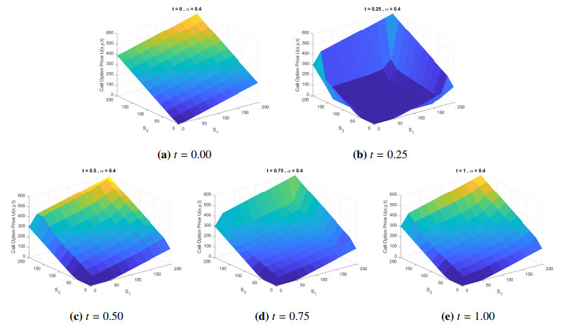
In this paper, we considered the two-dimensional fractional-order Black-Scholes model in the Liouville-Caputo sense. The Black-Scholes model was an important tool in the financial market, used for determining option prices in the European-style market. However, finding a closed-form analytical solution for the fractional-order partial differential equation was challenging. To address this, we introduced an improved finite difference method for approximating the solution of the two-dimensional fractional-order Black-Scholes model in the Liouville-Caputo sense, based on the Crank-Nicolson finite difference method. This method combined the concepts of the finite difference method for solving the multidimensional Black-Scholes model and the finite difference method for solving the fractional-order heat equation. We analyzed the conditional stability and the order of convergence. Furthermore, numerical examples were provided to illustrate the determination of option prices.
Citation: Din Prathumwan, Thipsuda Khonwai, Narisara Phoochalong, Inthira Chaiya, Kamonchat Trachoo. An improved approximate method for solving two-dimensional time-fractional-order Black-Scholes model: a finite difference approach[J]. AIMS Mathematics, 2024, 9(7): 17205-17233. doi: 10.3934/math.2024836
In this paper, we considered the two-dimensional fractional-order Black-Scholes model in the Liouville-Caputo sense. The Black-Scholes model was an important tool in the financial market, used for determining option prices in the European-style market. However, finding a closed-form analytical solution for the fractional-order partial differential equation was challenging. To address this, we introduced an improved finite difference method for approximating the solution of the two-dimensional fractional-order Black-Scholes model in the Liouville-Caputo sense, based on the Crank-Nicolson finite difference method. This method combined the concepts of the finite difference method for solving the multidimensional Black-Scholes model and the finite difference method for solving the fractional-order heat equation. We analyzed the conditional stability and the order of convergence. Furthermore, numerical examples were provided to illustrate the determination of option prices.

| [1] |
R. Almeida, M. Guzowska, T. Odzijewicz, A remark on local fractional calculus and ordinary derivatives, Open Math., 14 (2016), 1122–1124. https://doi.org/10.1515/math-2016-0104 doi: 10.1515/math-2016-0104

|
| [2] |
S. Kumar, D. Kumar, S. Abbasbandy, M. M. Rashidi, Analytical solution of fractional Navier-Stokes equation by using modified Laplace decomposition method, Ain Shams Eng. J., 5 (2014), 569–574. https://doi.org/10.1016/j.asej.2013.11.004 doi: 10.1016/j.asej.2013.11.004
|
| [3] |
Q. Huang, R. Zhdanov, Symmetries and exact solutions of the time fractional Harry-Dym equation with Riemann-Liouville derivative, Phys. A, 409 (2014), 110–118. https://doi.org/10.1016/j.physa.2014.04.043 doi: 10.1016/j.physa.2014.04.043
|
| [4] |
W. T. Chen, X. Xu, S. P. Zhu, Analytically pricing double barrier options based on a time-fractional Black-Scholes equation, Comput. Math. Appl., 69 (2015), 1407–1419. https://doi.org/10.1016/j.camwa.2015.03.025 doi: 10.1016/j.camwa.2015.03.025
|
| [5] |
M. Senol, O. Tasbozan, A. Kurt, Numerical solutions of fractional Burgers' type equations with conformable derivative, Chinese J. Phys., 58 (2019), 75–84. https://doi.org/10.1016/j.cjph.2019.01.001 doi: 10.1016/j.cjph.2019.01.001
|
| [6] | T. Mathur, S. Agarwal, S. P. Goyal, K. S. Pritam, Analytical solutions of some fractional diffusion boundary value problems, In: Fractional order systems and applications in engineering, Academic Press, 2023, 37–50. https://doi.org/10.1016/B978-0-32-390953-2.00010-4 |
| [7] |
E. Bonyah, M. L. Juga, C. W. Chukwu, Fatmawati, A fractional order dengue fever model in the context of protected travelers, Alex. Eng. J., 61 (2022), 927–936. https://doi.org/10.1016/j.aej.2021.04.070 doi: 10.1016/j.aej.2021.04.070
|
| [8] |
M. Mandal, S. Jana, S. K. Nandi, T. K. Kar, Modelling and control of a fractional-order epidemic model with fear effect, Energ. Ecol. Environ., 5 (2020), 421–432. https://doi.org/10.1007/s40974-020-00192-0 doi: 10.1007/s40974-020-00192-0
|
| [9] |
W. C. Chen, Nonlinear dynamics and chaos in a fractional-order financial system, Chaos Solitons Fract., 36 (2008), 1305–1314. https://doi.org/10.1016/j.chaos.2006.07.051 doi: 10.1016/j.chaos.2006.07.051
|
| [10] |
C. J. Xu, C. Aouiti, M. X. Liao, P. L. Li, Z. X. Liu, Chaos control strategy for a fractional-order financial model, Adv. Differ. Equ., 2020 (2020), 1–17. https://doi.org/10.1186/s13662-020-02999-x doi: 10.1186/s13662-020-02999-x
|
| [11] |
Y. J. He, J. Peng, S. Zheng, Fractional-order financial system and fixed-time synchronization, Fractal Fract., 6 (2022), 1–21. https://doi.org/10.3390/fractalfract6090507 doi: 10.3390/fractalfract6090507
|
| [12] |
W. Gao, P. Veeresha, H. M. Baskonus, Dynamical analysis fractional-order financial system using efficient numerical methods, Appl. Math. Sci. Eng., 31 (2023), 2155152. https://doi.org/10.1080/27690911.2022.2155152 doi: 10.1080/27690911.2022.2155152
|
| [13] |
F. Black, M. Scholes, The pricing of options and corporate liabilities, J. Political Econ., 81 (1973), 637–654. https://doi.org/10.1086/260062 doi: 10.1086/260062
|
| [14] |
M. Alghalith, Pricing the American options using the Black-Scholes pricing formula, Phys. A, 507 (2018), 443–445. https://doi.org/10.1016/j.physa.2018.05.087 doi: 10.1016/j.physa.2018.05.087
|
| [15] |
J. Vecer, Black-Scholes representation for Asian options, Math. Finance, 24 (2014), 598–626. https://doi.org/10.1111/mafi.12012 doi: 10.1111/mafi.12012
|
| [16] |
A. S. V. Ravi Kanth, K. Aruna, Solution of time fractional Black-Scholes European option pricing equation arising in financial market, Nonlinear Eng., 5 (2016), 269–276. https://doi.org/10.1515/nleng-2016-0052 doi: 10.1515/nleng-2016-0052
|
| [17] |
A. Golbabai, O. Nikan, T. Nikazad, Numerical analysis of time fractional Black-Scholes European option pricing model arising in financial market, Comput. Appl. Math., 38 (2019), 1–24. https://doi.org/10.1007/s40314-019-0957-7 doi: 10.1007/s40314-019-0957-7
|
| [18] |
X. J. He, S. Lin, A fractional Black-Scholes model with stochastic volatility and European option pricing, Expert Syst. Appl., 178 (2021), 114983. https://doi.org/10.1016/j.eswa.2021.114983 doi: 10.1016/j.eswa.2021.114983
|
| [19] |
Z. W. Tian, S. Y. Zhai, Z. F. Weng, Compact finite difference schemes of the time fractional Black-Scholes model, J. Appl. Anal. Comput., 10 (2020), 904–919. https://doi.org/10.11948/20190148 doi: 10.11948/20190148
|
| [20] |
P. Roul, A high accuracy numerical method and its convergence for time-fractional Black-Scholes equation governing European options, Appl. Numer. Math., 151 (2020), 472–493. https://doi.org/10.1016/j.apnum.2019.11.004 doi: 10.1016/j.apnum.2019.11.004
|
| [21] |
J. Kaur, S. Natesan, A novel numerical scheme for time-fractional Black-Scholes PDE governing European options in mathematical finance, Numer. Algorithms, 94 (2023), 1519–1549. https://doi.org/10.1007/s11075-023-01545-6 doi: 10.1007/s11075-023-01545-6
|
| [22] |
G. Jumarie, Derivation and solutions of some fractional Black-Scholes equations in coarse-grained space and time. Application to Merton's optimal portfolio, Comput. Math. Appl., 59 (2010), 1142–1164. https://doi.org/10.1016/j.camwa.2009.05.015 doi: 10.1016/j.camwa.2009.05.015
|
| [23] |
S. M. Nuugulu, F. Gideon, K. C. Patidar, A robust numerical solution to a time-fractional Black-Scholes equation, Adv. Differ. Equ., 2021 (2021), 123. https://doi.org/10.1186/s13662-021-03259-2 doi: 10.1186/s13662-021-03259-2
|
| [24] |
V. Gülkaç, The homotopy perturbation method for the Black-Scholes equation, J. Stat. Comput. Simul., 80 (2010), 1349–1354. https://doi.org/10.1080/00949650903074603 doi: 10.1080/00949650903074603
|
| [25] |
A. A. Elbeleze, A. Kılıçman, B. M. Taib, Homotopy perturbation method for fractional Black-Scholes European option pricing equations using Sumudu transform, Math. Probl. Eng., 2013 (2013), 1–7. https://doi.org/10.1155/2013/524852 doi: 10.1155/2013/524852
|
| [26] |
S. R. Saratha, G. S. S. Krishnan, M. Bagyalakshmi, C. P. Lim, Solving Black-Scholes equations using fractional generalized homotopy analysis method, Comput. Appl. Math., 39 (2020), 1–35. https://doi.org/10.1007/s40314-020-01306-4 doi: 10.1007/s40314-020-01306-4
|
| [27] | Y. Achdou, O. Pironneau, Computational methods for option pricing, Philadelphia: SIAM, 2005. https://doi.org/10.1137/1.9780898717495 |
| [28] | H. J. Bungartz, A. Heinecke, D. Pflüger, S. Schraufstetter, Parallelizing a Black-Scholes solver based on finite elements and sparse grids, 2010 IEEE International Symposium on Parallel & Distributed Processing, Workshops and Phd Forum (IPDPSW), USA: Atlanta, 1–8. https://doi.org/10.1109/IPDPSW.2010.5470707 |
| [29] |
F. Soleymani, S. F. Zhu, RBF-FD solution for a financial partial-integro differential equation utilizing the generalized multiquadric function, Comput. Math. Appl., 82 (2021), 161–178. https://doi.org/10.1016/j.camwa.2020.11.010 doi: 10.1016/j.camwa.2020.11.010
|
| [30] |
Y. H. Chen, L. Wei, S. Cao, F. Liu, Y. L. Yang, Y. J. Cheng, Numerical solving for generalized Black-Scholes-Merton model with neural finite element method, Digit. Signal Process., 131 (2022), 103757. https://doi.org/10.1016/j.dsp.2022.103757 doi: 10.1016/j.dsp.2022.103757
|
| [31] | Z. Fei, Y. Goto, E. Kita, Solution of Black-Scholes equation by using RBF approximation, In: Frontiers of computational science, Berlin, Heidelberg: Springer, 2007,339–343. https://doi.org/10.1007/978-3-540-46375-7_53 |
| [32] | J. F. Zhou, X. M. Gu, Y. L. Zhao, H. Li, A fast compact difference scheme with unequal time-steps for the tempered time-fractional Black-Scholes model, Int. J. Comput. Math., 2023, 1–23. https://doi.org/10.1080/00207160.2023.2254412 |
| [33] |
T. Guillaume, On the multidimensional Black-Scholes partial differential equation, Ann. Oper. Res., 281 (2019), 229–251. https://doi.org/10.1007/s10479-018-3001-1 doi: 10.1007/s10479-018-3001-1
|
| [34] |
G. Chacón-Acosta, R. O. Salas, Projection of the two-dimensional Black-Scholes equation for options with underlying stock and strike prices in two different currencies, Rev. Mex. Fís., 68 (2022), 011401. https://doi.org/10.31349/RevMexFis.68.011401 doi: 10.31349/RevMexFis.68.011401
|
| [35] |
W. Chen, S. Wang, A 2nd-order ADI finite difference method for a 2D fractional Black-Scholes equation governing European two asset option pricing, Math. Comput. Simul., 171 (2020), 279–293. https://doi.org/10.1016/j.matcom.2019.10.016 doi: 10.1016/j.matcom.2019.10.016
|
| [36] |
J. Wang, S. Wen, M. Yang, W. Shao, Practical finite difference method for solving multi-dimensional Black-Scholes model in fractal market, Chaos Solitons Fract., 157 (2022), 111895. https://doi.org/10.1016/j.chaos.2022.111895 doi: 10.1016/j.chaos.2022.111895
|
| [37] | Y. Heo, H. Han, H. Jang, Y. Choi, J. Kim, Finite difference method for the two-dimensional Black-Scholes equation with a hybrid boundary condition J. Korean Soc. Ind. Appl. Math., 23 (2019), 19–30. https://doi.org/10.12941/jksiam.2019.23.019 |
| [38] |
F. Soleymani, S. F. Zhu, Error and stability estimates of a time-fractional option pricing model under fully spatial-temporal graded meshes, J. Comput. Appl. Math., 425 (2023), 115075. https://doi.org/10.1016/j.cam.2023.115075 doi: 10.1016/j.cam.2023.115075
|
| [39] |
I. Karatay, N. Kale, S. Bayramoglu, A new difference scheme for time fractional heat equations based on the Crank-Nicholson method, Fract. Calc. Appl. Anal., 16 (2013), 892–910. https://doi.org/10.2478/s13540-013-0055-2 doi: 10.2478/s13540-013-0055-2
|
| [40] |
D. Pak, C. Han, W. T. Hong, Iterative speedup by utilizing symmetric data in pricing options with two risky assets, Symmetry, 9 (2017), 1–16. https://doi.org/10.3390/sym9010012 doi: 10.3390/sym9010012
|
| [41] |
C. P. Li, D. L. Qian, Y. Q. Chen, On Riemann-Liouville and Caputo derivatives, Discrete Dyn. Nat. Soc., 2011 (2011), 1–15. https://doi.org/10.1155/2011/562494 doi: 10.1155/2011/562494
|
| [42] |
M. Caputo, Linear models of dissipation whose Q is almost frequency independent–Ⅱ, Geophys. J. Int., 13 (1967), 529–539. https://doi.org/10.1111/j.1365-246X.1967.tb02303.x doi: 10.1111/j.1365-246X.1967.tb02303.x
|
| [43] | F. Sabzikar, M. M. Meerschaert, J. H. Chen, Tempered fractional calculus, J. Comput. Phys., 293 (2015), 14–28. https://doi.org/10.1016/j.jcp.2014.04.024 |
| [44] |
T. M. Atanacković, S. Pilipović, D. Zorica, Properties of the Caputo-Fabrizio fractional derivative and its distributional settings, Fract. Calc. Appl. Anal., 21 (2018), 29–44. https://doi.org/10.1515/fca-2018-0003 doi: 10.1515/fca-2018-0003
|
| [45] |
A. Atangana, D. Baleanu, New fractional derivatives with nonlocal and non-singular kernel: theory and application to heat transfer model, Thermal Sci., 20 (2016), 763–769. https://doi.org/10.2298/TSCI160111018A doi: 10.2298/TSCI160111018A
|
| [46] |
S. Kumar, D. Kumar, J. Singh, Numerical computation of fractional Black-Scholes equation arising in financial market, Egyptian J. Basic Appl. Sci., 1 (2014), 177–183. https://doi.org/10.1016/j.ejbas.2014.10.003 doi: 10.1016/j.ejbas.2014.10.003
|
| [47] | M. Choudhry, 46–Options Ⅳ: Pricing models for bond options, In: The bond & money markets, Butterworth-Heinemann, 2001,794–800. https://doi.org/10.1016/B978-075064677-2.50054-1 |
| [48] | M. Glantz, R. Kissell, Equity derivatives in multi-asset risk modeling, In: Multi-asset risk modeling, Academic Press, 2014,189–215. https://doi.org/10.1016/B978-0-12-401690-3.00006-8 |
| [49] |
P. Sawangtong, K. Trachoo, W. Sawangtong, B. Wiwattanapataphee, The analytical solution for the Black-Scholes equation with two assets in the Liouville-Caputo fractional derivative sense, Mathematics, 6 (2018), 1–14. https://doi.org/10.3390/math6080129 doi: 10.3390/math6080129
|
| [50] |
D. Prathumwan, K. Trachoo, On the solution of two-dimensional fractional Black-Scholes equation for European put option, Adv. Differ. Equ., 2020 (2020), 146. https://doi.org/10.1186/s13662-020-02554-8 doi: 10.1186/s13662-020-02554-8
|


Figures(4) / Tables(4)

Din Prathumwan, Thipsuda Khonwai, Narisara Phoochalong, Inthira Chaiya, Kamonchat Trachoo. An improved approximate method for solving two-dimensional time-fractional-order Black-Scholes model: a finite difference approach[J]. AIMS Mathematics, 2024, 9(7): 17205-17233. doi: 10.3934/math.2024836


 DownLoad: