Existence, and Ulam's types stability of higher-order fractional Langevin equations on a star graph

Gang Chen; Jinbo Ni; Xinyu Fu; Gang Chen; Jinbo Ni; Xinyu Fu

doi:10.3934/math.2024581

AIMS Mathematics

2024, Volume 9, Issue 5: 11877-11909. doi: 10.3934/math.2024581

Previous Article Next Article

Research article

Existence, and Ulam's types stability of higher-order fractional Langevin equations on a star graph

School of mathematics and big data, Anhui University of Science and Technology, Huainan 232001, China

Received: 25 January 2024 Revised: 07 March 2024 Accepted: 22 March 2024 Published: 26 March 2024
MSC : 34A08, 34A34, 34B15

A study was conducted on the existence of solutions for a class of nonlinear Caputo type higher-order fractional Langevin equations with mixed boundary conditions on a star graph with $ k+1 $ nodes and $ k $ edges. By applying a variable transformation, a system of fractional differential equations with mixed boundary conditions and different domains was converted into an equivalent system with identical boundary conditions and domains. Subsequently, the existence and uniqueness of solutions were verified using Krasnoselskii's fixed point theorem and Banach's contraction principle. In addition, the stability results of different types of solutions for the system were further discussed. Finally, two examples are illustrated to reinforce the main study outcomes.
- fractional Langevin equation,
- mixed boundary condition,
- existence and uniqueness,
- Ulam stability
Citation: Gang Chen, Jinbo Ni, Xinyu Fu. Existence, and Ulam's types stability of higher-order fractional Langevin equations on a star graph[J]. AIMS Mathematics, 2024, 9(5): 11877-11909. doi: 10.3934/math.2024581

Related Papers:

Abstract

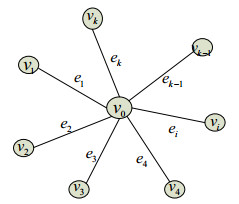
A study was conducted on the existence of solutions for a class of nonlinear Caputo type higher-order fractional Langevin equations with mixed boundary conditions on a star graph with $ k+1 $ nodes and $ k $ edges. By applying a variable transformation, a system of fractional differential equations with mixed boundary conditions and different domains was converted into an equivalent system with identical boundary conditions and domains. Subsequently, the existence and uniqueness of solutions were verified using Krasnoselskii's fixed point theorem and Banach's contraction principle. In addition, the stability results of different types of solutions for the system were further discussed. Finally, two examples are illustrated to reinforce the main study outcomes.

References

[1]	A. Kilbas, H. Srivastava, J. Trujillo, Theory and applications of fractional differential equations, Amsterdam: Elsevier Science Ltd., 2006.
[2]	S. Alizadeh, D. Baleanu, S. Rezapour, Analyzing transient response of the parallel RCL circuit by using the Caputo-Fabrizio fractional derivative, Adv. Differ. Equ., 2020 (2020), 55. https://doi.org/10.1186/s13662-020-2527-0 doi: 10.1186/s13662-020-2527-0
[3]	S. Rezapour, S. Etemad, H. Mohammadi, A mathematical analysis of a system of Caputo-Fabrizio fractional differential equations for the anthrax disease model in animals, Adv. Differ. Equ., 2020 (2020), 481. https://doi.org/10.1186/s13662-020-02937-x doi: 10.1186/s13662-020-02937-x
[4]	C. Li, R. Wu, R. Ma, Existence of solutions for caputo fractional iterative equations under several boundary value conditions, AIMS Mathematics, 8 (2023), 317–339. https://doi.org/10.3934/math.2023015 doi: 10.3934/math.2023015
[5]	B. Ahmad, M. Alghanmi, A. Alsaedi, J. Nieto, Existence and uniqueness results for a nonlinear coupled system involving caputo fractional derivatives with a new kind of coupled boundary conditions, Appl. Math. Lett., 116 (2021), 107018. https://doi.org/10.1016/j.aml.2021.107018 doi: 10.1016/j.aml.2021.107018
[6]	J. Ni, J. Zhang, W. Zhang, Existence of solutions for a coupled system of $p$-Laplacian Caputo-Hadamard fractional Sturm-Liouville-Langevin equations with antiperiodic boundary conditions, J. Math., 2022 (2022), 3346115. https://doi.org/10.1155/2022/3346115 doi: 10.1155/2022/3346115
[7]	A. Salem, B. Alghamdi, Multi-strip and multi-point boundary conditions for fractional Langevin equation, Fractal Fract., 4 (2020), 18. https://doi.org/10.3390/fractalfract4020018 doi: 10.3390/fractalfract4020018
[8]	Y. Adjabi, M. Samei, M. Matar, J. Alzabut, Langevin differential equation in frame of ordinary and Hadamard fractional derivatives under three point boundary conditions, AIMS Mathematics, 6 (2021), 2796–2843. https://doi.org/10.3934/math.2021171 doi: 10.3934/math.2021171
[9]	G. Lumer, Connecting of local operators and evolution equations on networks, In: Potential theory Copenhagen 1979, Berlin: Springer, 2006,219–234. https://doi.org/10.1007/BFb0086338
[10]	J. Graef, L. Kong, M. Wang, Existence and uniqueness of solutions for a fractional boundary value problem on a graph, FCAA, 17 (2014), 499–510. https://doi.org/10.2478/s13540-014-0182-4 doi: 10.2478/s13540-014-0182-4
[11]	V. Mehandiratta, M. Mehra, G. Leugering, Existence and uniqueness results for a nonlinear Caputo fractional boundary value problem on a star graph, J. Math. Anal. Appl., 477 (2019), 1243–1264. https://doi.org/10.1016/j.jmaa.2019.05.011 doi: 10.1016/j.jmaa.2019.05.011
[12]	S. Etemad, S. Rezapour, On the existence of solutions for fractional boundary value problems on the ethane graph, Adv. Differ. Equ., 2020 (2020), 276. https://doi.org/10.1186/s13662-020-02736-4 doi: 10.1186/s13662-020-02736-4
[13]	G. Mophou, G. Leugering, P. Fotsing, Optimal control of a fractional Sturm-Liouville problem on a star graph, Optimization, 70 (2021), 659–687. https://doi.org/10.1080/02331934.2020.1730371 doi: 10.1080/02331934.2020.1730371
[14]	A. Turab, Z. Mitrovi$\acute{c}$, A. Savi$\acute{c}$, Existence of solutions for a class of nonlinear boundary value problems on the hexasilinane graph, Adv. Differ. Equ., 2021 (2021), 494. https://doi.org/10.1186/s13662-021-03653-w doi: 10.1186/s13662-021-03653-w
[15]	X. Han, H. Cai, H. Yang, Existence and uniqueness of solutions for the boundary value problems of nonlinear fractional differential equations on star graph (Chinese), Acta Math. Sci., 42 (2022), 139–156.
[16]	W. Ali, A. Turab, J. Nieto, On the novel existence results of solutions for a class of fractional boundary value problems on the cyclohexane graph, J. Inequal. Appl., 2022 (2022), 5. https://doi.org/10.1186/s13660-021-02742-4 doi: 10.1186/s13660-021-02742-4
[17]	W. Zhang, J. Zhang, J. Ni, Existence and uniqueness results for fractional Langevin equations on a star graph, Math. Biosci. Eng., 19 (2022), 9636–9657. https://doi.org/10.3934/mbe.2022448 doi: 10.3934/mbe.2022448
[18]	D. Baleanu, S. Etemad, H. Mohammadi, S. Rezapour, A novel modeling of boundary value problems on the glucose graph, Commun. Nonlinear Sci., 100 (2021), 105844. https://doi.org/10.1016/j.cnsns.2021.105844 doi: 10.1016/j.cnsns.2021.105844
[19]	V. Mehandiratta, M. Mehra, G. Leugering, Existence results and stability analysis for a nonlinear fractional boundary value problem on a circular ring with an attached edge: A study of fractional calculus on metric graph, Netw. Heterog. Media., 16 (2021), 155–185. https://doi.org/10.3934/nhm.2021003 doi: 10.3934/nhm.2021003
[20]	H. Khan, Y. Li, W. Chen, D. Baleanu, A. Khan, Existence theorems and Hyers-Ulam stability for a coupled system of fractional differential equations with $p$-Laplacian operator, Bound. Value. Probl., 2017 (2017), 157. https://doi.org/10.1186/s13661-017-0878-6 doi: 10.1186/s13661-017-0878-6
[21]	H. Khan, F. Jarad, T. Abdeljawad, A. Khan, A singular ABC-fractional differential equation with $p$-Laplacian operator, Chaos Soliton. Fract., 129 (2019), 56–61. https://doi.org/10.1016/j.chaos.2019.08.017 doi: 10.1016/j.chaos.2019.08.017
[22]	A. Devi, A. Kumar, T. Abdeljawad, A. Khan, Stability analysis of solutions and existence theory of fractional Lagevin equation, Alex. Eng. J., 60 (2021), 3641–3647. https://doi.org/10.1016/j.aej.2021.02.011 doi: 10.1016/j.aej.2021.02.011
[23]	W. Zhang, W. Liu, Existence and Ulam's type stability results for a class of fractional boundary value problems on a star graph, Math. Method. Appl. Sci., 43 (2020), 8568–8594. https://doi.org/10.1002/mma.6516 doi: 10.1002/mma.6516
[24]	A. Devi, A. Kumar, Hyers-Ulam stability and existence of solution for hybrid fractional differential equation with $p$-Laplacian operator, Chaos Soliton. Fract., 156 (2022), 111859. https://doi.org/10.1016/j.chaos.2022.111859 doi: 10.1016/j.chaos.2022.111859
[25]	M. Abbas, Ulam stability and existence results for fractional differential equations with hybrid proportional-Caputo derivatives, J. Interdiscip. Math., 25 (2022), 213–231. https://doi.org/10.1080/09720502.2021.1889156 doi: 10.1080/09720502.2021.1889156
[26]	I. Ahmad, K. Shah, G. Ur Rahman, D. Baleanu, Stability analysis for a nonlinear coupled system of fractional hybrid delay differential equations, Math. Method. Appl. Sci., 43 (2020), 8669–8682. https://doi.org/10.1002/mma.6526 doi: 10.1002/mma.6526
[27]	I. Podlubny, Fractional differential equations: an introduction to fractional derivatives, fractional differential equations, to methods of their solution and some of their applications, San Diego: Academic Press, Inc., 1999.
[28]	C. Urs, Coupled fixed point theorems and applications to periodic boundary value problems, Miskolc Math. Notes, 14 (2013), 323–333. https://doi.org/10.18514/MMN.2013.598 doi: 10.18514/MMN.2013.598
[29]	A. Granas, J. Dugundji, Fixed point theory, New York: Springer, 2003. https://doi.org/10.1007/978-0-387-21593-8

Reader Comments

Your name:*

Email:*
© 2024 the Author(s), licensee AIMS Press. This is an open access article distributed under the terms of the Creative Commons Attribution License (http://creativecommons.org/licenses/by/4.0)