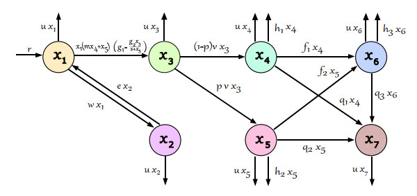
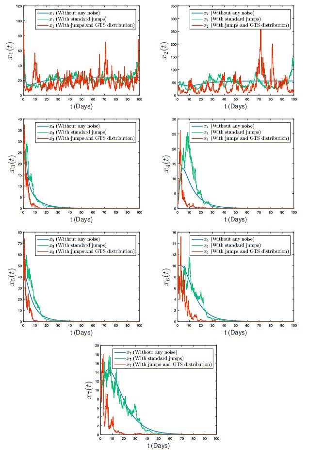
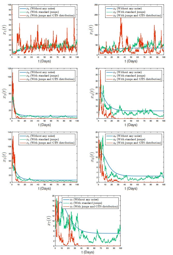
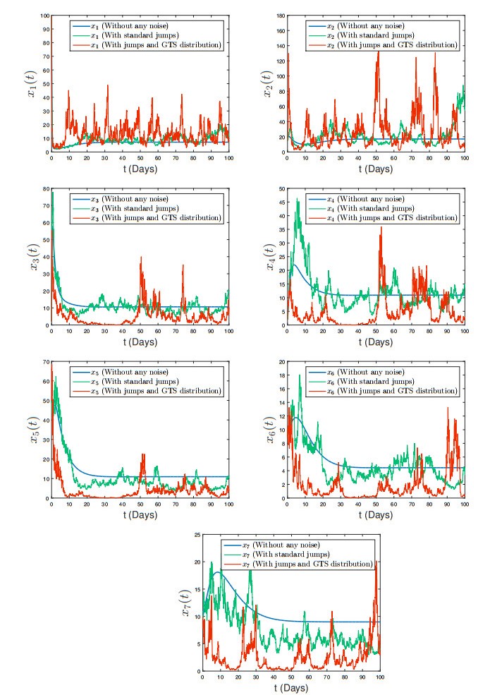
The generalized tempered stable (GTS) distribution is an optimal choice for modeling disease propagation, as it effectively captures the heavy-tailed nature of such events. This attribute is crucial for evaluating the impact of large-scale outbreaks and formulating effective public health interventions. In our study, we introduce a comprehensive stochastic epidemic model that incorporates various intervention strategies and utilizes Lévy jumps characterized by the GTS distribution. Notably, our proposed stochastic system does not exhibit endemic or disease-free states, challenging the conventional approach of assessing disease persistence or extinction based on asymptotic behavior. To address this, we employed a novel stochastic analysis approach to demonstrate the potential for disease eradication or continuation. We provide numerical examples to highlight the importance of incorporating the GTS distribution in epidemiological modeling. These examples validate the accuracy of our results and compare our model's outcomes with those of a standard system using basic Lévy jumps. The purposeful use of the GTS distribution accounts for the heavy-tailed nature of disease incidence or vector abundance, enhancing the precision of models and predictions in epidemiology.
Citation: Yassine Sabbar, Aeshah A. Raezah, Mohammed Moumni. Enhancing epidemic modeling: exploring heavy-tailed dynamics with the generalized tempered stable distribution[J]. AIMS Mathematics, 2024, 9(10): 29496-29528. doi: 10.3934/math.20241429
The generalized tempered stable (GTS) distribution is an optimal choice for modeling disease propagation, as it effectively captures the heavy-tailed nature of such events. This attribute is crucial for evaluating the impact of large-scale outbreaks and formulating effective public health interventions. In our study, we introduce a comprehensive stochastic epidemic model that incorporates various intervention strategies and utilizes Lévy jumps characterized by the GTS distribution. Notably, our proposed stochastic system does not exhibit endemic or disease-free states, challenging the conventional approach of assessing disease persistence or extinction based on asymptotic behavior. To address this, we employed a novel stochastic analysis approach to demonstrate the potential for disease eradication or continuation. We provide numerical examples to highlight the importance of incorporating the GTS distribution in epidemiological modeling. These examples validate the accuracy of our results and compare our model's outcomes with those of a standard system using basic Lévy jumps. The purposeful use of the GTS distribution accounts for the heavy-tailed nature of disease incidence or vector abundance, enhancing the precision of models and predictions in epidemiology.

| [1] | R. May, Stability and complexity in model ecosystems, Princeton: Princeton University Press, 2019. |
| [2] |
W. Kermack, A. McKendrick, A contribution to the mathematical theory of epidemics, Proc. R. Soc. Lond. A, 115 (1927), 700–721. http://dx.doi.org/10.1098/rspa.1927.0118 doi: 10.1098/rspa.1927.0118

|
| [3] |
Z. Wang, K. Tang, Combating COVID-19: health equity matters, Nat. Med., 26 (2020), 458. http://dx.doi.org/10.1038/s41591-020-0823-6 doi: 10.1038/s41591-020-0823-6
|
| [4] |
M. Hossain, The effect of the Covid-19 on sharing economy activities, J. Clean. Prod., 280 (2021), 124782. http://dx.doi.org/10.1016/j.jclepro.2020.124782 doi: 10.1016/j.jclepro.2020.124782
|
| [5] |
M. Roy, R. Holt, Effects of predation on host–pathogen dynamics in SIR models, Theor. Popul. Biol., 73 (2008), 319–331. http://dx.doi.org/10.1016/j.tpb.2007.12.008 doi: 10.1016/j.tpb.2007.12.008
|
| [6] |
Z. Neufeld, H. Khataee, A. Czirok, Targeted adaptive isolation strategy for COVID-19 pandemic, Infectious Disease Modelling, 5 (2020), 357–361. http://dx.doi.org/10.1016/j.idm.2020.04.003 doi: 10.1016/j.idm.2020.04.003
|
| [7] |
B. Buonomo, Effects of information-dependent vaccination behavior on coronavirus outbreak: insights from a SIRI model, Ricerche Mat., 69 (2020), 483–499. http://dx.doi.org/10.1007/s11587-020-00506-8 doi: 10.1007/s11587-020-00506-8
|
| [8] | H. Guo, M. Li, Z. Shuai, Global stability of the endemic equilibrium of multigroup SIR epidemic models, Canadian Applied Mathematics Quarterly, 14 (2006), 259–284. |
| [9] |
M. Mehdaoui, A. Alaoui, M. Tilioua, Analysis of a stochastic SVIR model with time-delayed stages of vaccination and Lévy jumps, Math. Method. Appl. Sci., 46 (2023), 12570–12590. http://dx.doi.org/10.1002/mma.9198 doi: 10.1002/mma.9198
|
| [10] |
E. Tornatore, S. Buccellato, P. Vetro, Stability of a stochastic SIR system, Physica A, 354 (2005), 111–126. http://dx.doi.org/10.1016/j.physa.2005.02.057 doi: 10.1016/j.physa.2005.02.057
|
| [11] | J. Jia, J. Ding, S. Liu, G. Liao, J. Li, B. Duan, et al., Modeling the control of COVID-19: impact of policy interventions and meteorological factors, arXiv: 2003.02985. http://dx.doi.org/10.48550/arXiv.2003.02985 |
| [12] |
D. Heymann, N. Shindo, COVID-19: what is next for public health? The Lancet, 395 (2020), 542–545. http://dx.doi.org/10.1016/S0140-6736(20)30374-3 doi: 10.1016/S0140-6736(20)30374-3
|
| [13] |
S. Bentout, Y. Chen, S. Djilali, Global dynamics of an SEIR model with two age structures and a nonlinear incidence, Acta Appl. Math., 171 (2021), 7. http://dx.doi.org/10.1007/s10440-020-00369-z doi: 10.1007/s10440-020-00369-z
|
| [14] |
H. Azizi, E. Esmaeili, Challenges and potential solutions in the development of COVID-19 pandemic control measures, New Microbes and New Infections, 40 (2021), 100852. http://dx.doi.org/10.1016/j.nmni.2021.100852 doi: 10.1016/j.nmni.2021.100852
|
| [15] |
D. Kiouach, Y. Sabbar, Modeling the impact of media intervention on controlling the diseases with stochastic perturbations, AIP Conf. Proc., 2074 (2019), 020026. http://dx.doi.org/10.1063/1.5090643 doi: 10.1063/1.5090643
|
| [16] |
Y. Sabbar, Asymptotic extinction and persistence of a perturbed epidemic model with different intervention measures and standard Lévy jumps, Bulletin of Biomathematics, 1 (2023), 58–77. http://dx.doi.org/10.59292/bulletinbiomath.2023004 doi: 10.59292/bulletinbiomath.2023004
|
| [17] |
D. Kiouach, Y. Sabbar, Stability and threshold of a stochastic SIRS epidemic model with vertical transmission and transfer from infectious to susceptible individuals, Discrete Dyn. Nat. Soc., 2018 (2018), 7570296. http://dx.doi.org/10.1155/2018/7570296 doi: 10.1155/2018/7570296
|
| [18] |
Y. Sabbar, M. Mehdaoui, M. Tilioua, K. Nisar, Probabilistic analysis of a disturbed SIQP-SI model of mosquito-borne diseases with human quarantine strategy and independent Poisson jumps, Model. Earth Syst. Environ., 10 (2024), 4695–4715. http://dx.doi.org/10.1007/s40808-024-02018-y doi: 10.1007/s40808-024-02018-y
|
| [19] |
M. Li, H. Smith, L. Wang, Global dynamics of an SEIR epidemic model with vertical transmission, SIAM J. Appl. Math., 62 (2001), 58–69. http://dx.doi.org/10.1137/S0036139999359860 doi: 10.1137/S0036139999359860
|
| [20] | F. Brauer, Compartmental models in epidemiology, In: Mathematical epidemiology, Berlin: Springer, 2008, 19–79. http://dx.doi.org/10.1007/978-3-540-78911-6_2 |
| [21] |
K. Roosa, Y. Lee, R. Luo, A. Kirpich, R. Rothenberg, J. Hyman, et al., Real-time forecasts of the COVID-19 epidemic in China from February 5th to February 24th, 2020, Infectious Disease Modelling, 5 (2020), 256–263. http://dx.doi.org/10.1016/j.idm.2020.02.002 doi: 10.1016/j.idm.2020.02.002
|
| [22] |
H. Aghdaouia, A. Raezahb, M. Tiliouaa, Y. Sabbara, Exploring COVID-19 model with general fractional deriva-tives: novel physics-informed-neural-networks approach for dynamics and order estimation, J. Math. Computer Sci., 36 (2025), 142–162. http://dx.doi.org/10.22436/jmcs.036.02.01 doi: 10.22436/jmcs.036.02.01
|
| [23] |
Vivek, M. Kumar, S. Mishra, Study of the spreading behavior of the biological SIR Model of COVID-19 disease through a fast fibonacci wavelet-based computational approach, Int. J. Appl. Comput. Math., 10 (2024), 106. http://dx.doi.org/10.1007/s40819-024-01699-4 doi: 10.1007/s40819-024-01699-4
|
| [24] |
L. Kalachev, J. Graham, E. Landguth, A simple modification to the classical SIR model to estimate the proportion of under-reported infections using case studies in flu and COVID-19, Infectious Disease Modelling, 9 (2024), 1147–1162. http://dx.doi.org/10.1016/j.idm.2024.06.002 doi: 10.1016/j.idm.2024.06.002
|
| [25] |
A. Kumar, T. Choi, S. Wamba, S. Gupta, K. Tan, Infection vulnerability stratification risk modelling of COVID-19 data: a deterministic SEIR epidemic model analysis, Ann. Oper. Res., 339 (2024), 1177–1203. http://dx.doi.org/10.1007/s10479-021-04091-3 doi: 10.1007/s10479-021-04091-3
|
| [26] |
G. Battineni, N. Chintalapudi, F. Amenta, SARS-CoV-2 epidemic calculation in Italy by SEIR compartmental models, Applied Computing and Informatics, 20 (2024), 251–261. http://dx.doi.org/10.1108/ACI-09-2020-0060 doi: 10.1108/ACI-09-2020-0060
|
| [27] |
R. Yousif, A. Jeribi, S. Al-Azzawi, Fractional-order SEIRD model for global COVID-19 outbreak, Mathematics, 11 (2023), 1036. http://dx.doi.org/10.3390/math11041036 doi: 10.3390/math11041036
|
| [28] |
D. Kiouach, S. El-idrissi, Y. Sabbar, Asymptotic behavior analysis and threshold sharpening of a staged progression AIDS/HIV epidemic model with Lévy jumps, Discontinuity, Nonlinearity, and Complexity, 12 (2023), 583–613. http://dx.doi.org/10.5890/DNC.2023.09.008 doi: 10.5890/DNC.2023.09.008
|
| [29] |
D. Lu, L. Sang, S. Du, T. Li, Y. Chang, X. Yang, Asymptomatic COVID-19 infection in late pregnancy indicated no vertical transmission, J. Med. Virol., 92 (2020), 1660–1664. http://dx.doi.org/10.1002/jmv.25927 doi: 10.1002/jmv.25927
|
| [30] |
D. Schwartz, A. Dhaliwal, Infections in pregnancy with COVID-19 and other respiratory RNA virus diseases are rarely, if ever, transmitted to the fetus: experiences with coronaviruses, parainfluenza, metapneumovirus respiratory syncytial virus, and influenza, Arch. Pathol. Lab. Med., 144 (2020), 920–928. http://dx.doi.org/10.5858/arpa.2020-0211-SA doi: 10.5858/arpa.2020-0211-SA
|
| [31] |
C. Xu, S. Yuan, T. Zhang, Competitive exclusion in a general multi-species chemostat model with stochastic perturbations, Bull. Math. Biol., 83 (2021), 4. http://dx.doi.org/10.1007/s11538-020-00843-7 doi: 10.1007/s11538-020-00843-7
|
| [32] |
B. Berrhazi, M. El Fatini, A. Laaribi, R. Pettersson, R. Taki, A stochastic SIRS epidemic model incorporating media coverage and driven by Lévy noise, Chaos Soliton. Fract., 105 (2017), 60–68. http://dx.doi.org/10.1016/j.chaos.2017.10.007 doi: 10.1016/j.chaos.2017.10.007
|
| [33] |
K. Bao, Q. Zhang, L. Rong, X. Li, Dynamics of an imprecise SIRS model with Lévy jumps, Physica A, 520 (2019), 489–506. http://dx.doi.org/10.1016/j.physa.2019.01.027 doi: 10.1016/j.physa.2019.01.027
|
| [34] |
M. Lakhal, R. Taki, M. El Fatini, T. El Guendouz, Quarantine alone or in combination with treatment measures to control COVID-19, J. Anal., 31 (2023), 2347–2369. http://dx.doi.org/10.1007/s41478-023-00569-4 doi: 10.1007/s41478-023-00569-4
|
| [35] |
M. Lakhal, T. Guendouz, R. Taki, M. El Fatini, The threshold of a stochastic SIRS epidemic model with a general incidence, Bull. Malays. Math. Sci. Soc., 47 (2024), 100. http://dx.doi.org/10.1007/s40840-024-01696-2 doi: 10.1007/s40840-024-01696-2
|
| [36] | A. Mdaghri, M. Lakhal, R. Taki, M. Fatini, Ergodicity and stationary distribution of a stochastic SIRI epidemic model with logistic birth and saturated incidence rate, J. Anal., in press. http://dx.doi.org/10.1007/s41478-024-00780-x |
| [37] |
J. Rosinski, Tempering stable processes, Stoch. Proc. Appl., 117 (2007), 677–707. http://dx.doi.org/10.1016/j.spa.2006.10.003 doi: 10.1016/j.spa.2006.10.003
|
| [38] | E. Jouini, J. Cvitanić, M. Musiela, Option pricing, interest rates and risk management, Cambridge: Cambridge University Press, 2001. http://dx.doi.org/10.1017/CBO9780511569708 |
| [39] |
S. Boyarchenko, S. Levendorskiǐ, Option pricing for truncated Lévy processes, Int. J. Theor. Appl. Fin., 3 (2000), 549–552. http://dx.doi.org/10.1142/S0219024900000541 doi: 10.1142/S0219024900000541
|
| [40] |
U. Küchler, S. Tappe, Bilateral gamma distributions and processes in financial mathematics, Stoch. Proc. Appl., 118 (2008), 261–283. http://dx.doi.org/10.1016/j.spa.2007.04.006 doi: 10.1016/j.spa.2007.04.006
|
| [41] |
I. Koponen, Analytic approach to the problem of convergence of truncated Lévy flights towards the Gaussian stochastic process, Phys. Rev. E, 52 (1995), 1197. http://dx.doi.org/10.1103/PhysRevE.52.1197 doi: 10.1103/PhysRevE.52.1197
|
| [42] |
P. Carr, H. Geman, D. Madan, M. Yor, The fine structure of asset returns: an empirical investigation, Journal of Business, 75 (2002), 305–332. http://dx.doi.org/10.1086/338705 doi: 10.1086/338705
|
| [43] |
D. Kiouach, Y. Sabbar, S. El-idrissi, New results on the asymptotic behavior of an SIS epidemiological model with quarantine strategy, stochastic transmission, and Lévy disturbance, Math. Method. Appl. Sci., 44 (2021), 13468–13492. http://dx.doi.org/10.1002/mma.7638 doi: 10.1002/mma.7638
|
| [44] | X. Mao, Stochastic differential equations and applications, Oxford: Woodhead Publishing Limited, 2007. |
| [45] | I. Karatzas, S. Shreve, Brownian motion and stochastic calculus, New York: Springer, 2014. http://dx.doi.org/10.1007/978-1-4612-0949-2 |
| [46] |
Y. Althobaity, M. Tildesley, Modelling the impact of non-pharmaceutical interventions on the spread of COVID-19 in Saudi Arabia, Sci. Rep., 13 (2023), 843. http://dx.doi.org/10.1038/s41598-022-26468-5 doi: 10.1038/s41598-022-26468-5
|
| [47] |
Z. Zhao, J. Wu, F. Cai, S. Zhang, Y. Wang, A hybrid deep learning framework for air quality prediction with spatial autocorrelation during the COVID-19 pandemic, Sci. Rep., 13 (2023), 1015. http://dx.doi.org/10.1038/s41598-023-28287-8 doi: 10.1038/s41598-023-28287-8
|
| [48] |
S. Ma, S. Li, J. Zhang, Spatial and deep learning analyses of urban recovery from the impacts of COVID-19, Sci. Rep., 13 (2023), 2447. http://dx.doi.org/10.1038/s41598-023-29189-5 doi: 10.1038/s41598-023-29189-5
|
Figures(5) / Tables(1)

Yassine Sabbar, Aeshah A. Raezah, Mohammed Moumni. Enhancing epidemic modeling: exploring heavy-tailed dynamics with the generalized tempered stable distribution[J]. AIMS Mathematics, 2024, 9(10): 29496-29528. doi: 10.3934/math.20241429


 DownLoad: