Prescribed-time adaptive stabilization of high-order stochastic nonlinear systems with unmodeled dynamics and time-varying powers

Yihang Kong; Xinghui Zhang; Yaxin Huang; Ancai Zhang; Jianlong Qiu; Yihang Kong; Xinghui Zhang; Yaxin Huang; Ancai Zhang; Jianlong Qiu

doi:10.3934/math.20241380

AIMS Mathematics

2024, Volume 9, Issue 10: 28447-28471. doi: 10.3934/math.20241380

Previous Article Next Article

Research article Special Issues

Prescribed-time adaptive stabilization of high-order stochastic nonlinear systems with unmodeled dynamics and time-varying powers

1.
School of Automation and Electrical Engineering, Linyi University, Linyi, 276000, China
2.
School of Information Science and Engineering, Shandong Normal University, Jinan, 250014, China

Received: 26 July 2024 Revised: 13 September 2024 Accepted: 29 September 2024 Published: 08 October 2024
MSC : 93D05, 93E15

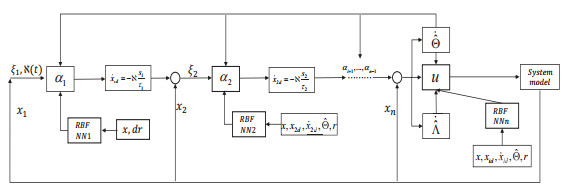
In this paper, the control problem of prescribed-time adaptive neural stabilization for a class of non-strict feedback stochastic high-order nonlinear systems with dynamic uncertainty and unknown time-varying powers is discussed. The parameter separation technique, dynamic surface control technique, and dynamic signals were used to eradicate the influences of unknown time-varying powers together with state and input unmodeled dynamics, and to mitigate the computational intricacy of the backstepping. In a non-strict feedback framework, the radial basis function neural networks (RBFNNs) and Young's inequality were deployed to reconstruct the continuous unknown nonlinear functions. Finally, by establishing a new criterion of stochastic prescribed-time stability and introducing a proper bounded control gain function, an adaptive neural prescribed-time state-feedback controller was designed, ensuring that all signals of the closed-loop system were semi-global practical prescribed-time stable in probability. A numerical example and a practical example successfully validated the productivity and superiority of the control scheme.
Citation: Yihang Kong, Xinghui Zhang, Yaxin Huang, Ancai Zhang, Jianlong Qiu. Prescribed-time adaptive stabilization of high-order stochastic nonlinear systems with unmodeled dynamics and time-varying powers[J]. AIMS Mathematics, 2024, 9(10): 28447-28471. doi: 10.3934/math.20241380

Related Papers:

Abstract

In this paper, the control problem of prescribed-time adaptive neural stabilization for a class of non-strict feedback stochastic high-order nonlinear systems with dynamic uncertainty and unknown time-varying powers is discussed. The parameter separation technique, dynamic surface control technique, and dynamic signals were used to eradicate the influences of unknown time-varying powers together with state and input unmodeled dynamics, and to mitigate the computational intricacy of the backstepping. In a non-strict feedback framework, the radial basis function neural networks (RBFNNs) and Young's inequality were deployed to reconstruct the continuous unknown nonlinear functions. Finally, by establishing a new criterion of stochastic prescribed-time stability and introducing a proper bounded control gain function, an adaptive neural prescribed-time state-feedback controller was designed, ensuring that all signals of the closed-loop system were semi-global practical prescribed-time stable in probability. A numerical example and a practical example successfully validated the productivity and superiority of the control scheme.

References

[1]	S. Bhat, D. Bernstein, Finite-time stability of continuous autonomous systems, SIAM J. Control Optim., 38 (2000), 751–766. https://doi.org/10.1137/s0363012997321358 doi: 10.1137/s0363012997321358
[2]	A. Polyakov, D. Efimov, W. Perruquetti, Finite-time and fixed-time stabilization: Implicit Lyapunov function approach, Automatica, 51 (2015), 332–340. https://doi.org/10.1016/j.automatica.2014.10.082 doi: 10.1016/j.automatica.2014.10.082
[3]	J. T. Hu, G. X. Sui, X. X. Lu, X. D. Li, Fixed-time control of delayed neural networks with impulsive perturbations, Nonlinear Anal. Model., 23 (2018), 904–920. https://doi.org/10.15388/na.2018.6.6 doi: 10.15388/na.2018.6.6
[4]	D. B. Tong, B. Ma, Q. Y. Chen, Y. B. Wei, P. Shi, Finite-time synchronization and energy consumption prediction for multilayer fractional-order networks, IEEE T. Circuits II, 70 (2023), 2176–2180. https://doi.org/10.1109/tcsii.2022.3233420 doi: 10.1109/tcsii.2022.3233420
[5]	G. Q. Yang, D. B. Tong, Q. Y. Chen, W. N. Zhou, Fixed-time synchronization and energy consumption for Kuramoto-oscillator networks with multilayer distributed control, IEEE T. Circuits II, 70 (2023), 1555–1559. https://doi.org/10.1109/tcsii.2022.3221477 doi: 10.1109/tcsii.2022.3221477
[6]	K. Ding, Q. X. Zhu, T. W. Huang, Prefixed-time local intermittent sampling synchronization of stochastic multicoupling delay reaction-diffusion dynamic networks, IEEE T. Neur. Net. Lear., 35 (2024), 718–732. https://doi.org/10.1109/TNNLS.2022.3176648 doi: 10.1109/TNNLS.2022.3176648
[7]	H. Wang, Q. X. Zhu, Global stabilization of a class of stochastic nonlinear time-delay systems with SISS inverse dynamics, IEEE T. Automat. Contr., 65 (2020), 4448–4455. https://doi.org/10.1109/tac.2020.3005149 doi: 10.1109/tac.2020.3005149
[8]	J. Yu, S. Cheng, P. Shi, C. Lin, Command-filtered neuroadaptive output-feedback control for stochastic nonlinear systems with input constraint, IEEE T. Cybernetics, 53 (2023), 2301–2310. https://doi.org/10.1109/TCYB.2021.3115785 doi: 10.1109/TCYB.2021.3115785
[9]	Z. C. Zhu, Q. X. Zhu, Adaptive event-triggered fuzzy control for stochastic highly nonlinear systems with time delay and nontriangular structure interconnections, IEEE T. Fuzzy Syst., 32 (2024), 27–37. https://doi.org/10.1109/TFUZZ.2023.3287869 doi: 10.1109/TFUZZ.2023.3287869
[10]	F. Wang, B. Chen, Y. Sun, Y. Gao, C. Lin, Finite-time fuzzy control of stochastic nonlinear systems, IEEE T. Cybernetics, 50 (2020), 2617–2626. https://doi.org/10.1109/TCYB.2019.2925573 doi: 10.1109/TCYB.2019.2925573
[11]	H. Min, S. Xu, Z. Zhang, Adaptive finite-time stabilization of stochastic nonlinear systems subject to full-state constraints and input saturation, IEEE T. Automat. Contr., 66 (2021), 1306–1313. https://doi.org/10.1109/TAC.2020.2990173 doi: 10.1109/TAC.2020.2990173
[12]	K. Li, Y. Li, G. Zong, Adaptive fuzzy fixed-time decentralized control for stochastic nonlinear systems, IEEE T. Fuzzy Syst., 29 (2021), 3428–3440. https://doi.org/10.1109/TFUZZ.2020.3022570 doi: 10.1109/TFUZZ.2020.3022570
[13]	Y. G. Yao, J. Q. Tan, J. Wu, X. Zhang, Event-triggered fixed-time adaptive fuzzy control for state-constrained stochastic nonlinear systems without feasibility conditions, Nonlinear Dyn., 105 (2021), 403–416. https://doi.org/10.1007/s11071-021-06633-7 doi: 10.1007/s11071-021-06633-7
[14]	H. Peng, Q. X. Zhu, Fixed time stability of impulsive stochastic nonlinear time-varying systems, Int. J. Robust Nonlin., 33 (2023), 3699–3714. https://doi.org/10.1002/rnc.6589 doi: 10.1002/rnc.6589
[15]	Y. Song, Y. Wang, J. Holloway, M. Krstic, Time-varying feedback for regulation of normal-form nonlinear systems in prescribed finite time, Automatica, 83 (2017), 243–251. https://doi.org/10.1016/j.automatica.2017.06.008 doi: 10.1016/j.automatica.2017.06.008
[16]	W. Q. Li, M. Krstic, Stochastic nonlinear prescribed-time stabilization and inverse optimality, IEEE T. Automat. Contr., 67 (2022), 1179–1193. https://doi.org/10.1109/TAC.2021.3061646 doi: 10.1109/TAC.2021.3061646
[17]	W. Li, M. Krstic, Prescribed-time control of stochastic nonlinear systems with reduced control effort, J. Syst. Sci. Complex, 34 (2021), 1782–1800. https://doi.org/10.1007/s11424-021-1217-7 doi: 10.1007/s11424-021-1217-7
[18]	W. Q. Li, M. Krstic, Prescribed-time output-feedback control of stochastic nonlinear systems, IEEE T. Automat. Contr., 68 (2023), 1431–1446. https://doi.org/10.1109/TAC.2022.3151587 doi: 10.1109/TAC.2022.3151587
[19]	H. Wang, Q. X. Zhu, Finite-time stabilization of high-order stochastic nonlinear systems in strict-feedback form, Automatica, 54 (2015), 284–291. https://doi.org/10.1016/j.automatica.2015.02.016 doi: 10.1016/j.automatica.2015.02.016
[20]	L. Zhang, X. Liu, C. Hua, Prescribed-time control for stochastic high-order nonlinear systems with parameter uncertainty, IEEE T. Circuits II, 70 (2023), 4083–4087. https://doi.org/10.1109/TCSII.2023.3274680 doi: 10.1109/TCSII.2023.3274680
[21]	J. Z. Liu, S. Yan, D. L. Zeng, Y. Hu, Y. Lv, A dynamic model used for controller design of a coal fired once-through boiler-turbine unit, Energy, 93 (2015), 2069–2078. https://doi.org/10.1016/j.energy.2015.10.077 doi: 10.1016/j.energy.2015.10.077
[22]	G. J. Li, X. J. Xie, Adaptive state-feedback stabilization of stochastic high-order nonlinear systems with time-varying powers and stochastic inverse dynamics, IEEE T. Automat. Contr., 65 (2020), 5360–5367. https://doi.org/10.1109/TAC.2020.2969547 doi: 10.1109/TAC.2020.2969547
[23]	F. Shen, X. Wang, X. Yin, Adaptive control based on Barrier Lyapunov function for a class of full-state constrained stochastic nonlinear systems with dead-zone and unmodeled dynamics, T. I. Meas. Control, 43 (2021), 1936–1948. https://doi.org/10.1177/01423312209856 doi: 10.1177/01423312209856
[24]	X. Xia, J. Pan, T. Zhang, Command filter based adaptive DSC of uncertain stochastic nonlinear systems with input delay and state constraints, J. Franklin I., 359 (2022), 9492–9521. https://doi.org/10.1016/j.jfranklin.2022.10.004 doi: 10.1016/j.jfranklin.2022.10.004
[25]	Y. Chen, Y. J. Liu, L. Liu, Event-triggered adaptive stabilization control of stochastic nonlinear systems with unmodeled dynamics, Int. J. Robust Nonlin., 33 (2023), 5322–5336. https://doi.org/10.1002/rnc.6645 doi: 10.1002/rnc.6645
[26]	Y. Shu, Neural dynamic surface control for stochastic nonlinear systems with unknown control directions and unmodelled dynamics, IET Control Theory A., 17 (2023), 649–661. https://doi.org/10.1049/cth2.12221 doi: 10.1049/cth2.12221
[27]	Y. C. Liu, Q. D. Zhu, X. Fan, Event-triggered adaptive fuzzy control for stochastic nonlinear time-delay systems, Fuzzy set. syst., 452 (2023), 42–60. https://doi.org/10.1016/j.fss.2022.07.005 doi: 10.1016/j.fss.2022.07.005
[28]	Y. C. Liu, Q. D. Zhu, Adaptive neural network asymptotic control design for MIMO nonlinear systems based on event-triggered mechanism, Inform. Sciences, 603 (2022), 91–105. https://doi.org/10.1016/j.ins.2022.04.048 doi: 10.1016/j.ins.2022.04.048
[29]	R. H. Cui, X. J. Xie, Finite-time stabilization of stochastic low-order nonlinear systems with time-varying orders and FT-SISS inverse dynamics, Automatica, 125 (2021), 109418. https://doi.org/10.1016/j.automatica.2020.109418 doi: 10.1016/j.automatica.2020.109418
[30]	Y. Liu, Y. Li, W. Li, Output-feedback stabilization of a class of stochastic nonlinear systems with time-varying powers, Int. J. Robust Nonlin., 31 (2021), 9175–9192. https://doi.org/10.1002/rnc.5761 doi: 10.1002/rnc.5761
[31]	H. Li, W. Li, J. Gu, Adaptive tracking control of stochastic nonlinear systems with unknown time-varying powers, J. Intel. Mat. Syst. Str., 43 (2021), 1880–1890. https://doi.org/10.1177/014233122098223 doi: 10.1177/014233122098223
[32]	W. Li, Y. Liu, X. Yao, State-feedback stabilization and inverse optimal control for stochastic high-order nonlinear systems with time-varying powers, Asian J. Control, 23 (2021), 739–750. https://doi.org/10.1002/asjc.2250 doi: 10.1002/asjc.2250
[33]	J. Gu, H. Wang, W. Li, Adaptive state-feedback stabilization for stochastic nonlinear systems with time-varying powers and unknown covariance, Mathematics, 10 (2022), 2873. https://doi.org/10.3390/math10162873 doi: 10.3390/math10162873
[34]	Y. Song, J. Su, A unified Lyapunov characterization for finite time control and prescribed time control, Int. J. Robust Nonlin., 33 (2023), 2930–2949. https://doi.org/10.1002/rnc.6544 doi: 10.1002/rnc.6544
[35]	Y. C. Liu, Q. D. Zhu, Adaptive neural network finite-time tracking control of full state constrained pure feedback stochastic nonlinear systems, J. Franklin I., 357 (2020), 6738–6759. https://doi.org/10.1016/j.jfranklin.2020.04.048 doi: 10.1016/j.jfranklin.2020.04.048
[36]	R. Khasminskii, Stochastic stability of differential equations, Berlin: Springer, 2011. https://doi.org/10.1007/978-3-642-23280-0
[37]	Z. P. Jiang, L. Praly, Design of robust adaptive controllers for nonlinear systems with dynamic uncertainties, Automatica, 34 (1998), 825–840. https://doi.org/10.1016/S0005-1098(98)00018-1 doi: 10.1016/S0005-1098(98)00018-1
[38]	M. Arcak, P. Kokotovic, Robust nonlinear control of systems with input unmodeled dynamics, Syst. Control Lett., 41 (2000), 115–122. https://doi.org/10.1016/S0167-6911(00)00044-X doi: 10.1016/S0167-6911(00)00044-X
[39]	F. C. Kong, H. L. Ni, Q. X. Zhu, C. Hu, T. W. Huang, Fixed-time and predefined-time synchronization of discontinuous neutral-type competitive networks via non-chattering adaptive control strategy, IEEE T. Netw. Sci. Eng., 10 (2023), 3644–3657. https://doi.org/10.1109/tnse.2023.3271109 doi: 10.1109/tnse.2023.3271109
[40]	C. C. Chen, C. J. Qian, X. Z. Lin, Z. Y. Sun, Y. W. Liang, Smooth output feedback stabilization for a class of nonlinear systems with time-varying powers, Int. J. Robust Nonlin., 27 (2017), 5113–5128. https://doi.org/10.1002/rnc.3826 doi: 10.1002/rnc.3826
[41]	Q. Chen, D. Tong, W. Zhou, Finite-time stochastic boundedness for Markovian jumping systems via the sliding mode control, J. Franklin I., 359 (2022), 4678–4698. https://doi.org/10.1016/j.jfranklin.2022.05.005 doi: 10.1016/j.jfranklin.2022.05.005
[42]	S. Sui, C. L. P. Chen, S. Tong, Event-trigger-based finite-time fuzzy adaptive control for stochastic nonlinear system with unmodeled dynamics, IEEE T. Fuzzy Syst., 29 (2021), 1914–1926. https://doi.org/10.1109/TFUZZ.2020.2988849 doi: 10.1109/TFUZZ.2020.2988849
[43]	R. M. Sanner, J. J. E. Slotine, Gaussian networks for direct adaptive control, In: 1991 American Control Conference, 1991, 2153–2159. https://doi.org/10.23919/ACC.1991.4791778
[44]	H. K. Khalil, Nonlinear systems, 2002.

Reader Comments

Your name:*

Email:*
© 2024 the Author(s), licensee AIMS Press. This is an open access article distributed under the terms of the Creative Commons Attribution License (http://creativecommons.org/licenses/by/4.0)