


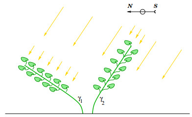
Figure 1.
A stem γ1 perpendicular to the sun rays is optimally shaped to collect the most light. For the stem γ2 bending toward the light source, the upper leaves put the lower ones in shade.
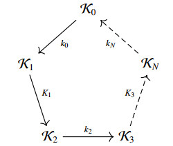
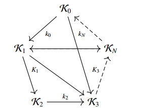
In this article, a new type of generalized, self-evolving and efficient automated statement proof algorithm based on new data structures, i.e., brackets and map graphs, and new algorithms is presented. The brackets structure provides an elegant low-knowledge representation of mathematical concepts. The map graphs offer an efficient machine-learning method which let the computer learn knowledge while proving. Additionally, the new finding is built completely on category theory. Furthermore, a prototype of the program is presented and examined for performance.
Citation: Zijian Wang, Xinhui Shao. A new type of generic, self-evolving and efficient automated deduction algorithm based on category theory[J]. AIMS Mathematics, 2023, 8(8): 18278-18294. doi: 10.3934/math.2023929
| [1] | Jingjing Yang, Jianqiu Lu . Stabilization in distribution of hybrid stochastic differential delay equations with Lévy noise by discrete-time state feedback controls. AIMS Mathematics, 2025, 10(2): 3457-3483. doi: 10.3934/math.2025160 |
| [2] | Xiao Yu, Yan Hua, Yanrong Lu . Observer-based robust preview tracking control for a class of continuous-time Lipschitz nonlinear systems. AIMS Mathematics, 2024, 9(10): 26741-26764. doi: 10.3934/math.20241301 |
| [3] | Hany Bauomy . Control and optimization mechanism of an electromagnetic transducer model with nonlinear magnetic coupling. AIMS Mathematics, 2025, 10(2): 2891-2929. doi: 10.3934/math.2025135 |
| [4] | Jenjira Thipcha, Presarin Tangsiridamrong, Thongchai Botmart, Boonyachat Meesuptong, M. Syed Ali, Pantiwa Srisilp, Kanit Mukdasai . Robust stability and passivity analysis for discrete-time neural networks with mixed time-varying delays via a new summation inequality. AIMS Mathematics, 2023, 8(2): 4973-5006. doi: 10.3934/math.2023249 |
| [5] | Limei Liu, Xitong Zhong . Analysis and anti-control of period-doubling bifurcation for the one-dimensional discrete system with three parameters and a square term. AIMS Mathematics, 2025, 10(2): 3227-3250. doi: 10.3934/math.2025150 |
| [6] | Abdul Qadeer Khan, Zarqa Saleem, Tarek Fawzi Ibrahim, Khalid Osman, Fatima Mushyih Alshehri, Mohamed Abd El-Moneam . Bifurcation and chaos in a discrete activator-inhibitor system. AIMS Mathematics, 2023, 8(2): 4551-4574. doi: 10.3934/math.2023225 |
| [7] | Zhiqiang Chen, Alexander Yurievich Krasnov . Disturbance observer based fixed time sliding mode control for a class of uncertain second-order nonlinear systems. AIMS Mathematics, 2025, 10(3): 6745-6763. doi: 10.3934/math.2025309 |
| [8] | Sheng-Ran Jia, Wen-Juan Lin . Adaptive event-triggered reachable set control for Markov jump cyber-physical systems with time-varying delays. AIMS Mathematics, 2024, 9(9): 25127-25144. doi: 10.3934/math.20241225 |
| [9] | Hyung Tae Choi, Jung Hoon Kim . An L∞ performance control for time-delay systems with time-varying delays: delay-independent approach via ellipsoidal D-invariance. AIMS Mathematics, 2024, 9(11): 30384-30405. doi: 10.3934/math.20241466 |
| [10] | Nasser. A. Saeed, Amal Ashour, Lei Hou, Jan Awrejcewicz, Faisal Z. Duraihem . Time-delayed control of a nonlinear self-excited structure driven by simultaneous primary and 1:1 internal resonance: analytical and numerical investigation. AIMS Mathematics, 2024, 9(10): 27627-27663. doi: 10.3934/math.20241342 |
In this article, a new type of generalized, self-evolving and efficient automated statement proof algorithm based on new data structures, i.e., brackets and map graphs, and new algorithms is presented. The brackets structure provides an elegant low-knowledge representation of mathematical concepts. The map graphs offer an efficient machine-learning method which let the computer learn knowledge while proving. Additionally, the new finding is built completely on category theory. Furthermore, a prototype of the program is presented and examined for performance.
In the recent papers [7,9] two functionals were introduced, measuring the amount of light collected by the leaves, and the amount of water and nutrients collected by the roots of a tree. In connection with a ramified transportation cost [1,14,18], these lead to various optimization problems for tree shapes.
Quite often, optimal solutions to problems involving a ramified transportation cost exhibit a fractal structure [2,3,4,12,15,16,17]. In the present note we analyze in more detail the optimization problem for tree branches proposed in [7], in the 2-dimensional case. In this simple setting, the unique solution can be explicitly determined. Instead of being fractal, its shape reminds of a solar panel.
The present analysis was partially motivated by the goal of understanding phototropism, i.e., the tendency of plant stems to bend toward the source of light. Our results indicate that this behavior cannot be explained purely in terms of maximizing the amount of light collected by the leaves (Fig. 1). Apparently, other factors must have played a role in the evolution of this trait, such as the competition among different plants. See [6] for some results in this direction.
The remainder of this paper is organized as follows. In Section 2 we review the two functionals defining the shape optimization problem and state the main results. Proofs are then worked out in Sections 3 to 5. Finally, in Section 6 we show the sharpness of the assumptions used in Theorem 2.5 and discuss various possible extensions.
We begin by reviewing the two functionals considered in [7,9].
Let
| n∈Sd−1≐{x∈Rd;|x|=1}, |
and assume that all light rays come parallel to
| x=y+sn | (1) |
with
On the perpendicular subspace
| μn(A)=μ({x∈Rd;πn(x)∈A}). | (2) |
Call
Definition 2.1. The total amount of sunlight from the direction
| Sn(μ)≐∫E⊥n(1−exp{−Φn(y)})dy. | (3) |
More generally, given an integrable function
| Sη(μ)≐∫Sd−1(∫E⊥n(1−exp{−Φn(y)})dy)η(n)dn. | (4) |
In the formula (4),
Remark 1. According to the above definition, the amount of sunlight
Consider a positive Radon measure
Definition 2.2. A measurable map
| χ:Θ×R+↦Rd | (5) |
is called an admissible irrigation plan for the measure
(ⅰ) For every
| ˙χ(ξ,t)=∂∂tχ(ξ,t) |
the partial derivative w.r.t. time, one has
| |˙χ(ξ,t)|={1for a.e.t∈[0,T(ξ)],0fort>T(ξ). | (6) |
(ⅱ) At time
(ⅲ) The push-forward of the Lebesgue measure on
| μ(A)= meas({ξ∈Θ;χ(ξ,T(ξ))∈A}). | (7) |
One may think of
To define the corresponding transportation cost, we first compute how many particles travel through a point
| |x|χ≐meas({ξ∈Θ;χ(ξ,t)=xfor somet≥0}). | (8) |
We think of
Definition 2.3. For a given
| Eα(χ)≐∫Θ(∫T(ξ)0|χ(ξ,t)|α−1χdt)dξ. | (9) |
The
| Iα(μ)≐infχEα(χ), | (10) |
where the infimum is taken over all admissible irrigation plans for the measure
Remark 2. Sometimes it is convenient to consider more general irrigation plans where, in place of (6), for a.e.
| Eα(χ)≐∫Θ(∫T(ξ)0|χ(ξ,t)|α−1χ|˙χ(ξ,t)|dt)dξ. | (11) |
Of course, one can always re-parameterize each trajectory
Remark 3. In the case
| Eα(χ)≐∫Θ(∫R+|˙χt(ξ,t)|dt)dξ=∫Θ[total length of the pathχ(ξ,⋅)]dξ. |
Of course, this length is minimal if every path
| Iα(μ)≐infχEα(χ)=∫Θ|χ(ξ,T(ξ))|dξ=∫|x|dμ. |
On the other hand, when
For the basic theory of ramified transport we refer to the monograph [1]. For future use, we recall that optimal irrigation plans satisfy
Single Path Property. If
| χ(ξ,t)=χ(ξ′,t)forallt∈[0,τ]. | (12) |
Another property that will be repeatedly used in the sequel is the following.
Lemma 2.4. Let
| Eα(˜χ)≤Eα(χ). | (13) |
If
Proof. The first statement is obvious. As in Lemma 5.15 in [1], the inequality (13) follows from the fact that, in the projected irrigation plan, the length of particle trajectories decreases while the multiplicity increases. Indeed,
| Eα(˜χ)≐∫Θ(∫T(ξ)0|˜χ(ξ,t)|α−1˜χ|ddt˜χ(ξ,t)|dt)dξ=∫Θ(∫T(ξ)0|(pC∘χ)(ξ,t)|α−1pC∘χ|ddt(pC∘χ)(ξ,t)|dt)dξ≤∫Θ(∫T(ξ)0|χ(ξ,t)|α−1χ|˙χ(ξ,t)|dt)dξ=Eα(χ). |
Combining the two functionals (4) and (10), one can formulate an optimization problem for the shape of branches:
| Sη(μ)−cIα(μ). | (14) |
We consider here the optimization problem for branches in the planar case
| maximize:Sn(μ)−cIα(μ), | (15) |
over all positive measures
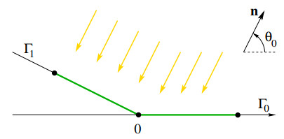
Theorem 2.5. In dimension
| Supp(μ)⊂{(rcosθ,rsinθ);r≥0,eitherθ=0orθ=θ0+π2}≐Γ0∪Γ1. | (16) |
When
| sinθ0≥1−22α−1. | (17) |
In the case
| Sn(˜μ)−cI1(˜μ)≥Sn(μ)−cI1(μ), |
with strict inequality if
In the case
Having proved that the optimal measure
| maximize:J0(u)≐∫+∞0sinθ0(1−e−u(s)/sinθ0)ds−c∫+∞0(∫+∞su(r)dr)αds. | (18) |
among all non-negative functions
We write (18) in the form
| maximize:J0(u)≐∫+∞0[sinθ0(1−e−u(s)/sinθ0)−czα]ds, | (19) |
subject to
| ˙z=−u,z(+∞)=0. | (20) |
The necessary conditions for optimality (see for example [8,11]) now yield
| u(s)=argmaxω≥0{−e−ω/sinθ0sinθ0−ωq(s)}=−(sinθ0)lnq(s), | (21) |
where the dual variable
| ˙q=cαzα−1,q(0)=0. | (22) |
Notice that, by (21),
| dz(q)dq=sinθ0cαz1−αlnq,z(1)=0. | (23) |
This equation admits the explicit solution
| z(q)=(sinθ0c)1/α[1+qlnq−q]1/α. | (24) |
Inserting (24) in (22), we obtain an implicit equation for
| s=(sinθ0)1−αααc1/α∫q(s)0[1+tlnt−t]1−ααdt. | (25) |
In turn, the density
| ℓ0=(sinθ0)1−αααc1/α∫10[1+slns−s]1−ααds. |
In particular, the total mass
| M0=∫ℓ00u(s)ds=z(0)=(sinθ0c)1/α. | (26) |
The density of the optimal measure along the ray
| ℓ1=1αc1/α∫10[1+slns−s]1−ααds, |
while the total mass is given by
| M1=c−1/α. | (27) |
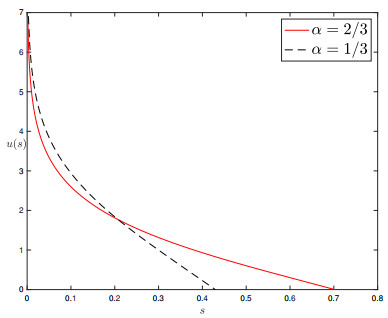
An illustration of how the corresponding density profile
In the analysis of the optimization problem (OPB), the case
When
Theorem 2.6. Let
| K≐max|w|=1∫n∈S1|⟨w,n⟩|η(n)dn. | (28) |
(i) If
(ii) If
A proof will be given in Section 5.
In this section we consider the optimization problem (15) in dimension
By the result in [7] we know that an optimal measure
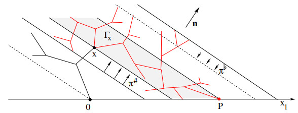
Next, consider the set of all branches, namely
| B≐{x∈R2+;|x|χ>0}. | (29) |
By the single path property, we can introduce a partial ordering among points in
| χ(t,ξ)=y⟹χ(t′,ξ)=xfor somet′∈[0,t]. | (30) |
This means that all particles that reach the point
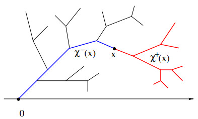
For a given
| χ−(x)≐{y∈B;y⪯x},χ+(x)≐{y∈B;x⪯y}, | (31) |
respectively (see Fig. 4).
We begin by deriving some properties of the sets
Lemma 3.1. Let the measure
| χ+(x)⊂Γx≐{y∈R2+;⟨n,y⟩∈[ax,bx]}, | (32) |
where
● If
● If
| bx=max{ax,b′x},b′x≐sup{⟨n,z⟩;z∈¯χ+(x)∩Re1}. |
Proof. The right-hand side of (32) is illustrated in Fig. 5. To prove the lemma, consider the set of all particles that pass through
| Θx≐{ξ∈[0,M];χ(τ,ξ)=xfor some τ≥0}. |
1. We first show that, by the optimality of the solution,
| ⟨n,χ(ξ,t)⟩≥axfor allξ∈Θx,t≥τ. | (33) |
Indeed, consider the perpendicular projection on the half plane
| π♯:R2↦S♯≐{y∈R2;⟨n,y⟩≥ax}. |
Define the projected irrigation plan
| χ♯(t,ξ)≐{π♯∘χ(t,ξ)ifξ∈Θx,t≥τ,χ(t,ξ)otherwise. |
Then the new measure
2. Next, we show that
| ⟨n,χ(ξ,t)⟩≤bxfor allξ∈Θxt≥τ. | (34) |
Indeed, call
| b″≐sup{⟨n,z⟩;z∈χ+(x)}. |
If
| π♭:R2↦S♭≐{y∈R2;⟨n,y⟩≤b″−δ}, |
one has
| {π♭(y);y∈χ+(x)}⊆R2+. | (35) |
Similarly as before, define the projected irrigation plan
| χ♭(t,ξ)≐{π♭∘χ(t,ξ)ifξ∈Θx,t≥τ,χ(t,ξ)otherwise. |
Then the new measure
Based on the previous lemma, we now consider the set
| B∗≐{x∈B;¯χ+(x)∩Re1≠∅}. | (36) |
It will be convenient to rotate coordinates by an angle of
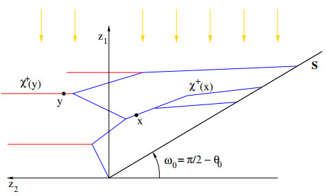
| S≐{(z1,z2);z1≥0,z2=−λz1},whereλ=tanθ0. | (37) |
Calling
Lemma 3.2. Let
(i) For every
(ii) If
| χ+(ˉz)⊂{(ˉz1,s);s∈R}. | (38) |
To make further progress, we define
| zmax1≐sup{z1;(z1,z2)∈B∗}. |
Moreover, on the interval
| φ(z1)≐sup{s;(z1,s)∈B∗}. | (39) |
Lemma 3.3. For every
Proof. 1. Assume that, on the contrary, for some
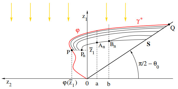
2. Choose two values
| −λˉz1<b<a<φ(ˉz1). |
By construction, for every
| Pn⪯An⪯Bn |
all in
| An=(tn,a),Bn=(t′n,b),ˉz1≤tn≤t′n≤zmax1. |
3. Since the total mass
| ∑n≥1|An|χ≤M≐μ(R2+). |
We can thus find
| c(b−a)αεα−1N>1. | (40) |
Consider the modified transport plan
| ˜Θ≐Θ∖{ξ;χ(ξ,τ)=BNfor someτ≥0}. |
Let
Calling
| Sn(μ)−Sn(˜μ)≤(μ−˜μ)(R2)=σ0. | (41) |
We now estimate the reduction in the transportation cost, achieved by replacing
| ∫sBsA|γ(s)|αχds−∫sBsA(|γ(s)|χ−σ0)αds≥(sB−sA)αsups|γ(s)|α−1χ⋅σ0≥(b−a)αεα−1Nσ0. |
This yields
| Iα(˜μ)≤Eα(˜χ)≤Iα(μ)−(b−a)αεα−1Nσ0. | (42) |
If (40) holds, combining (41)-(42) one obtains
| Sn(μ)−cIα(μ)<Sn(˜μ)−cIα(˜μ). |
Hence the measure
By the previous result, the graph of
Along the curve
Lemma 3.4. In the above setting, for every
| φ(s)<z2,jfor alls<z1,j. | (43) |
Proof. If (43) fails, there exists another point
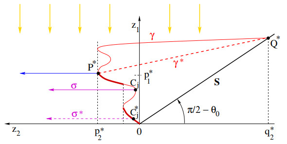
Next, as shown in Fig. 8, we consider a point
| p∗2=max{z2;(z1,z2)∈γ}≥0. | (44) |
Notice that such a maximum exists because
| p∗1=min{z1;(z1,p∗2)∈γ}. | (45) |
Moreover, call
| q∗2≐inf{z2;(z1,z2)∈Supp(μ)}, |
and let
| Σ∗≐{(z1,z2);z1∈[0,q∗1],z2≥q∗2}. |
Otherwise, call
| χ∗(ξ,t)≐π∗(χ(ξ,t)) |
is an irrigation plan for
| Sn(μ∗)=Sn(μ),Iα(μ∗)≤Eα(χ∗)<Eα(χ)=Iα(μ), |
contradicting the optimality assumption.
By a projection argument we now show that, in an optimal solution, all the particle paths remain below the segment
Lemma 3.5. In the above setting, let
| γ∗={(z1,z2);z1=a+bz2,z2∈[q∗2,p∗2]} |
be the segment with endpoints
| (ξ,t)↦χ(ξ,t)=(z1(ξ,t),z2(ξ,t)) | (46) |
is an optimal irrigation plan for the problem (15), then for a.e.
| z2(ξ,t)∈[q∗2,p∗2]⟹z1(ξ,t)≤a+bz2(ξ,t). | (47) |
Proof. 1. It suffices to show that the maximal curve
| Ω∗={ξ∈[0,M];χ(ξ,t∗)=P∗for some t∗≥0,z2(ξ,t)<p∗2for t>t∗}. | (48) |
Notice that, by the single path property (see Section 7.1 in [1]), all these particles follow the same path from the origin to
2. Consider the convex region below
| Σ≐{(z1,z2);0≤z1≤a+bz2,z2∈[q∗2,p∗2]}. |
Let
| χ†(ξ,t)≐{π(χ(ξ,t))ifξ∈Ω∗,t>t∗,χ(ξ,t)otherwise, | (49) |
has total cost strictly smaller than
| |π(x)|χ†≥|x|χ,|˙χ†(ξ,t)|≤|˙χ(ξ,t)|. | (50) |
Notice that, in (50), equality can hold for a.e.
3. We now observe that the perpendicular projection on
To address this issue, we observe that all particles
| z†2(ξ,t∗)=z2(ξ,t∗)=p∗2,z†2(ξ,T(ξ))≤z2(ξ,T(ξ))<p∗2. | (51) |
By continuity, for each
| z†2(ξ,τ(ξ))=z2(ξ,T(ξ)). |
Call
| ˜χ(ξ,t)≐{χ†(ξ,t)ifξ∈Ω∗,t≤τ(ξ),χ(ξ,τ(ξ))ifξ∈Ω∗,t≥τ(ξ),χ(ξ,t)ifξ∉Ω∗. | (52) |
By construction, the measures
| Eα(˜χ)≤Eα(χ†)<Eα(χ). |
This contradicts optimality, thus proving the lemma.
In this section we give a proof of Theorem 2.5. We recall that the functional (15) to be maximized is the difference between a payoff, i.e. the sunlight
As shown in Fig. 8, let
(ⅰ)
(ⅱ)
Assume that case (ⅰ) occurs. Then, by Lemma 3.4, the only branch that can bifurcate to the left of
The remainder of the proof will be devoted to showing that the case (ⅱ) cannot occur, because it would contradict the optimality of the solution.
To illustrate the heart of the matter, we first consider the elementary configuration shown in Fig. 9, left, where all trajectories are straight lines. Water is first transported from the origin to the point
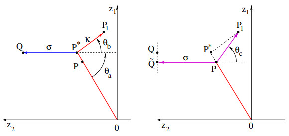
Next, as shown in Fig. 9, right, we consider a point
To fix ideas, we denote the lengths of the segments
| ℓa=|P−P∗|,ℓb=|P1−P∗|. | (53) |
The angles between these segments and a horizontal line will be denoted by
Lemma 4.1. Let
| cosθb>1−22α−1, | (54) |
or if
| Eα(˜χ)<Eα(χ). | (55) |
Proof. 1. To compute the difference between the quantities in (55), notice that the old transportation cost along
| (κ+σ)αℓa+καℓb |
is replaced by the new cost
| κα√ℓ2a+ℓ2b−2ℓaℓbcos(θa+θb)+σαℓacosθa. | (56) |
Notice that the last term in (56) accounts for the fact that an amount
The difference in the cost is thus expressed by the function
| f(ℓa,ℓb)=Eα(χ)−Eα(˜χ)=(κ+σ)αℓa−σαℓacosθa+κα[ℓb−√ℓ2a+ℓ2b−2ℓaℓbcos(θa+θb)]. |
2. Introducing the variables
| ε=ℓaℓb,ℓ=ℓb,εℓ=ℓa, |
we obtain
| f(εℓ,ℓ)=ℓ[ε(κ+σ)α−εσαcosθa+κα(1−√1+ε2−2εcos(θa+θb))]=εℓ[(κ+σ)α−σαcosθa+καcos(θa+θb)+O(1)⋅ε]. | (57) |
Setting
| λ=σκ+σ∈[0,1[, |
we are thus led to study the function
| F(λ,θa,θb)≐1−λαcosθa+(1−λ)αcos(θa+θb) | (58) |
and to find conditions which imply the positivity of
3. The function
| F(λ,θa,θb)=1−cosθa[λα−(1−λ)αcosθb]−sinθa(1−λ)αsinθb=1−⟨(cosθa,sinθa),(λα−(1−λ)αcosθb,(1−λ)αsinθb)⟩. | (59) |
To prove that
| λ2α+(1−λ)2α−2λα(1−λ)αcosθb<1. |
This inequality holds provided that
| cosθb>λ2α+(1−λ)2α−12λα(1−λ)α. | (60) |
Two cases must be considered. If
| λ2α+(1−λ)2α≤1for allλ∈[0,1]. |
Hence (60) trivially holds for all
On the other hand, if
| g(λ)≐λ2α+(1−λ)2α−12λα(1−λ)α=1+(λα−(1−λ)α)2−12λα(1−λ)α. |
We observe that, for
| 0≤g(λ)≤g(12)=1−22α−1, | (61) |
while
| limλ→0+g(λ)=limλ→1−g(λ)=0. |
From (61) it now follows that the condition (54) guarantees that (60) holds, hence
Summarizing the previous analysis, for any
(ⅰ) When
(ⅱ) When
4. Combining (57) with (58), we obtain
| f(θa,θb)=ℓa(κ+σ)α[F(λ,θa,θb)+O(1)⋅ℓaℓb]. | (62) |
By the previous step, in both cases (ⅰ) and (ⅱ) the right hand side of (62) is strictly positive provided that the ratio
We now consider a more general irrigation plan
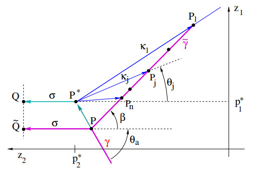
| 0≤θn<⋯<θ2<θ1, | (63) |
until they reach points
We compare this configuration with a modified irrigation plan
Lemma 4.2. Let the masses
| cosθ1>1−22α−1, | (64) |
or if
| Eα(χ)−Eα(˜χ)>0. | (65) |
Proof. 1. The left-hand side of (65), describing the difference between the old and the new transportation cost, can be expressed as
| |P−P∗|(σ+n∑j=1κj)α+n∑j=1καj|P∗−Pj|−σαcosθa|P−P∗|−n∑j=1(j∑i=1κi)α|Pj+1−Pj|, | (66) |
where, for notational convenience, we set
| Eα(χ)−Eα(˜χ)=A+Sn, | (67) |
where
| A≐|P−P∗|[(σ+n∑j=1κj)α−σαcosθa]+(n∑j=1κj)α(|P∗−P1|−|P−P1|), | (68) |
| Sn=n∑j=1καj|P∗−Pj|−(n∑j=1κj)α(|P∗−P1|−|Pn+1−P1|)−n∑j=1(j∑i=1κi)α|Pj+1−Pj|. | (69) |
2. Notice that the quantity
| A≥|P−P∗|[(σ+κ)α−σαcosθa+καcos(θa+θ1)−κα2|P−P∗||P1−P∗|]. | (70) |
Indeed, the last two terms within the square brackets in (70) are derived from
| |P∗−P1|−|P−P1|=|P∗−P1|[1−√1−2|P−P∗||P∗−P1|cos(θa+θ1)+|P−P∗|2|P∗−P1|2]≥|P∗−P1|[1−(1−|P−P∗||P∗−P1|cos(θa+θ1)+|P−P∗|22|P∗−P1|2)]. |
Using Lemma 4.1, we can now choose
| |P−P∗||P1−P∗|<ε′, | (71) |
then the right hand side of (70) is strictly positive. It now suffices to observe that, given all the angles
| β−θ1<ε⟹|P−P∗||P1−P∗|<ε′. | (72) |
In turn, this implies the strict inequality
| A>0. | (73) |
3. To complete the proof of the lemma, it remains to prove that
| |Pn−P1|≤|P∗−P1|,(n∑i=1κi)α≤καn+(n−1∑i=1κi)α, |
we obtain
| Sn=n∑j=1καj|P∗−Pj|−(n∑j=1κj)α(|P∗−P1|−|Pn−P1|)⏟≥0−n−1∑j=1(j∑i=1κi)α|Pj+1−Pj|≥καn|P∗−Pn|+n−1∑j=1καj|P∗−Pj|−(καn+(n−1∑j=1κj)α)(|P∗−P1|−|Pn−P1|)−(n−1∑i=1κi)α|Pn−Pn−1|−n−2∑j=1(j∑i=1κi)α|Pj+1−Pj|=n−1∑j=1καj|P∗−Pj|−(n−1∑j=1κj)α(|P∗−P1|−|Pn−1−P1|)−n−2∑j=1(j∑i=1κi)α|Pj+1−Pj|+καn(|P∗−Pn|+|Pn−P1|−|P∗−P1|)=Sn−1+καn(|P∗−Pn|−|P∗−P1|+|Pn−P1|)≥Sn−1, | (74) |
where in the second equality we have used
| Sn≥Sn−1≥⋯≥S1. |
Observing that
| S1=κα1|P∗−P1|−κα1(|P∗−P1|−|P2−P1|)−κα1|P2−P1|=0, |
the proof of the lemma is completed.
Remark 4. As soon as all the masses
| Eα(χ)−Eα(˜χ)>c0|P1−P∗|, | (75) |
for some
Let
As remarked at the beginning of this section, a proof of Theorem 2.5 can be achieved by showing that, for an optimal solution, the point
1. Call
| Θ∗≐{ξ∈Θ;χ(ξ,t∗)=P∗for somet∗>0} | (76) |
the set of particles that move through
| γ(0)=0,γ(t∗)=P∗,χ(ξ,t)=γ(t)for allξ∈Θ∗,t∈[0,t∗]. | (77) |
As a consequence, in (76) the time
Within the set
| Θ∗=Θl∪Θr. | (78) |
Here
| χ(t,ξ)∈{(z1,z2);z1≥p∗1,z2≤p∗2}. | (79) |
For future use, we denote
| σ≐meas(Θl),κ≐meas(Θr). | (80) |
2. In connection with the path
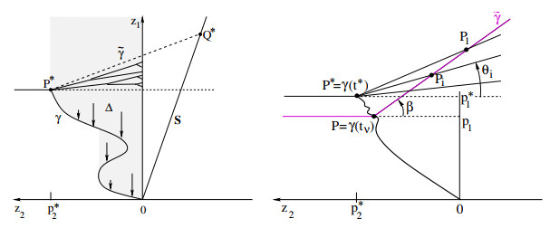
| Δ≐{(z1,z2);there existsˆz1<z1andt∈[0,t∗]such that(ˆz1,z2)=γ(t)}. | (81) |
We claim that the measure
| Sn(ˆμ)=Sn(μ),Iα(ˆμ)<Iα(μ), |
contradicting the optimality of
3. The previous argument shows that there are no sinks inside
| τ(ξ)≐min{t>t∗;χ(ξ,t)=(z1,0)for somez1≥p∗1}, |
and introduce the measure
| ˉμ(V)=meas{ξ∈Θr;χ(ξ,τ(ξ))∈V}. |
We observe that the restriction of
| {(ξ,t);ξ∈Θr,t∈[t∗,τ(ξ)]} |
yields an optimal transport plan from a point mass located at
By the interior regularity property (see Theorem 8.16 in [1], or Theorem 4.10 in [19]), outside a neighborhood of the support of
4. By the previous step, within a neighborhood of
Adopting the same notation used in Lemma 4.2, we call
| Θr=Θ1∪⋯∪Θn, | (82) |
where
We recall that, by Lemma 3.5, all particle paths
Case 1:
Case 2:
| cosθ1>cos(π2−θ0)=sinθ0≥1−22α−1. | (83) |
5. In this step, under the assumption that
For
| w(t)=γ(t)−γ(t∗)|γ(t)−γ(t∗)|. |
By compactness, there exists an increasing sequence
| limν→∞w(tν)=ˉw, | (84) |
for some unit vector
In connection with the masses
Next, we choose
A new measure
● The measure
| ϕ(z1,z2)={(p1,z2)ifz1=p∗1,z2>p∗2,(z1,z2)otherwise. |
● Recalling (78), for
● Particles
● Particles
6. By construction we have
| Θ†ν≐{ξ∈Θ∖Θ∗;χ(ξ,tν)=γ(tν)=P}. |
This is the set of particles that go through
We observe that, in the case where
| Iα(˜μ)≤Eα(˜χ)<Eα(χ)=Iα(μ). | (85) |
The following analysis will show that the same conclusion can still be reached, provided that
| δν≐meas(Θ†ν) | (86) |
is sufficiently small. For future use, we observe that
| limν→∞tν=t∗,limν→∞δν=0. | (87) |
We are now ready to estimate the difference between the two irrigation costs, in the general case.
(1) For
| χ(ξ,t)=˜χ(ξ,t),|χ(ξ,t)|χ=|˜χ(ξ,t)|˜χ | (88) |
for all
(2) For
| τ(ξ)=sup{t∈[tν,T(ξ)];χ(ξ,t)=γ(t)}<t∗ |
is the time when the particle
| A≐∫Θ†ν∫τ(ξ)tν(|˜χ(ξ,t)|α−1˜χ−|χ(ξ,t)|α−1χ)dtdξ≤∫Θ†ν∫τ(ξ)tν|˜χ(ξ,t)|α−1˜χdtdξ≤[meas(Θ†ν)]α⋅(t∗−tν). | (89) |
(3) It remains to estimate the difference in the cost for transporting particles
| B≐∫Θ∗(∫˜T(ξ)0|˜χ(ξ,t)|α−1˜χdt−∫T(ξ)0|χ(ξ,t)|α−1χdt)dξ. | (90) |
The estimate of
| B≤−c0|P1−P∗|. | (91) |
In the general case, recalling (86), the multiplicity along
| σ+κ≤|γ(t)|χ≤σ+κ+δνfor allt∈[tν,t∗]. |
The presence of the additional particles
| ∫Θ∗∫t∗tν[(σ+κ)α−1−(σ+κ+δν)α−1]dtdξ=[(σ+κ)α−1−(σ+κ+δν)α−1](σ+κ)(t∗−tν). | (92) |
On the other hand, the fact that the curve
| (σ+κ)⋅(σ+κ+δν)α−1⋅((t∗−tν)−|P∗−P|). | (93) |
Combining all the previous observations, from (89), (91), (92), and (93), we conclude
| Eα(˜χ)−Eα(χ)≤δαν(t∗−tν)−c0|P1−P∗|+[(σ+κ)α−1−(σ+κ+δν)α−1](σ+κ)(t∗−tν)−(σ+κ)⋅(σ+κ+δν)α−1⋅((t∗−tν)−|P∗−P|). | (94) |
We claim that, for some choice of
Case 1:
| Eα(˜χ)−Eα(χ)≤2δαν|γ(tν)−P∗|−c0|P1−P∗|+[(σ+κ)α−1−(σ+κ+δν)α−1]⋅2(σ+κ)|γ(tν)−P∗|. | (95) |
We now observe that the limit (84) implies an inequality of the form
| |γ(tν)−P∗|≤C|P1−P∗|, |
for a suitable constant
Case 2:
| Eα(˜χ)−Eα(χ)≤δαν(t∗−tν)+[(σ+κ)α−1−(σ+κ+δν)α−1](σ+κ)(t∗−tν)−(σ+κ)⋅(σ+κ+δν)α−1⋅12(t∗−tν). | (96) |
When
We give here a proof of Theorem 2.6.
1. Assume that there exists a unit vector
| K=∫n∈S1|⟨w∗,n⟩|η(n)dn>c. |
Let
Then the payoff achieved by
| Sη(μ)−cI0(μ)=ℓ⋅∫S1(1−exp{−λ|⟨w∗,n⟩|})|⟨w∗,n⟩|η(n)dn−cℓ |
| ≥ℓ⋅(1−e−λ)∫S1|⟨w∗,n⟩|η(n)dn−cℓ=[(1−e−λ)K−c]ℓ. | (97) |
By choosing
2. Next, assume that
| Sn(μ)≤∫ℓ0|⟨˙γ(s)⊥,n⟩|ds. |
Indeed, it is bounded by the length of the projection of
| Sη(μ)≤∫ℓ0∫S1|⟨˙γ(s)⊥,n⟩|η(n)dnds≤Kℓ. |
More generally,
| Sη(μ)≤∑iSη(μi)≤∑iKℓi. |
Hence
| Sη(μ)−cI0(μ)≤∑iKℓi−c∑iℓi≤0. |
This concludes the proof of case (ⅱ) in Theorem 2.6.
We first clarify the role of the assumption (17), used in Theorem 2.5 when
Consider the problem of irrigating two masses
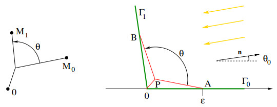
| cosθ=1−λ2α−(1−λ)2α2λα(1−λ)α,λ=M0M0+M1. | (98) |
For a proof, see Lemma 12.2 of [1]. As a consequence, we have the implications
| 12<α≤1⟹cosθ∈]0,22α−1−1],α=12⟹cosθ=0,0≤α<12⟹cosθ∈[22α−1−1,0[. |
Notice that
● When
● When
This is the underlying motivation for the assumption (17), repeatedly used in the proofs. Notice that a similar assumption (54) was introduced in Lemma 4.1.
It is interesting to speculate whether the conclusion of Theorem 2.5 may still hold when
| M0≐μ(Γ0)=(sinθ0c)1/α,M1=μ(Γ1)=(1c)1/α. | (99) |
Therefore
| λ=M0M0+M1=(sinθ0)1/α1+(sinθ0)1/α,sinθ0=λα(1−λ)α. | (100) |
In order for this configuration to be optimal, a necessary condition is
| cosθ=1−λ2α−(1−λ)2α2λα(1−λ)α≥cos(θ0+π2)=−sinθ0. | (101) |
Indeed, if (101) fails, a better configuration could be constructed as shown in Fig. 12, right. Here
The inequality (101) is precisely what is needed to rule out this possibility. Namely, if (101) holds, then the point
| 1−λ2α−(1−λ)2α2λα(1−λ)α≥−λα(1−λ)α. |
Equivalently:
| ϕ(λ)≐(1−λ)2α−λ2α−1≤0. | (102) |
We observe that
| ϕ′(λ)=−2α[(1−λ)2α−1+λ2α−1]<0 |
for
We conclude this paper by discussing possible extensions of our results.
(I) Motivated by the previous analysis, we conjecture that the conclusion of Theorem 2.5 remains valid even without the assumption (17). Namely, for all
(II) In Theorem 2.5 it was assumed that sunlight comes from one single direction. In the case considered at (4), where sunlight comes with varying intensity from different directions, one may conjecture that a similar result still holds true. This guess seems very reasonable if the support of the function
(III) It would be interesting to analyze the optimal branch configuration in three space dimensions. To fix ideas, assume that sunlight comes from the direction parallel to
| Γ0≐{v∈R3;⟨v,n⟩≥0,⟨v,e⟩=0},Γ1≐{v∈R3;⟨v,n⟩=0,⟨v,e⟩≥0}. |
In addition, the Hausdorff measure of Supp
The research of the first author was partially supported by NSF with grant DMS-1714237, "Models of controlled biological growth". The research of the second author was partially supported by a grant from the U.S.-Norway Fulbright Foundation.
| [1] | S. Wolfram, Wolfram language & system documentation center, Wolfram Research Inc., Champaign, IL, US, 12Eds., 2019. |
| [2] | X. S. Gao, Geoexpert, Beijing, 1998. Available from: http://www.mmrc.iss.ac.cn/gex/. |
| [3] |
L. D. Moura, S. Ullrich, The lean 4 theorem prover and programming language, Autom. Deduction -CADE, 2021,625–235. http://doi.org/10.1007/978-3-030-79876-5_37 doi: 10.1007/978-3-030-79876-5_37

|
| [4] | L. D. Moura, N. Bjørner, Z3: An efficient smt solver, In: Tools and Algorithms for the Construction and Analysis of Systems, 4963 (2008), 337–340. http://doi.org/10.1007/978-3-540-78800-3_24 |
| [5] | W. W. Li, Daishuxue Fangfa, 1 Ed, High Education Press, Beijing, 2019. ISBN 978-7-04-050725-6. |
| [6] | H. Ebbinghaus, Memory: A contribution to experimental psychology, Teachers College, Columbia University, New York City, 1913. Available from: https://archive.org/details/memorycontributi00ebbiuoft/page/n5/mode/2up. |
| [7] | K. Entacher, A collection of selected pseudorandom number generators with linear structures, 1997. Available from: https://www.semanticscholar.org/paper/6ae5fe88d296e70f188b0d12207d468c8f36e262. |
| [8] | A. S. Tanenbaum, Operating systems: Design and implementation (volume 1), Publishing House of Electronics Industry, Beijing, 3 Eds., 2015. ISBN 978-7-121-26193-0. |
| [9] | Z. J. Wang, The defqed repository, 2022. Available from: https://github.com/ZijianFelixWang/DefQed. |
| [10] | Z. J. Wang, Benchmark of the defqed algorithm, 2022. Available from: https://github.com/ZijianFelixWang/DefQed-Benchmark. |
| [11] | H. Packard, The hp zbook 14u g5 specifications, 2018. https://support.hp.com/us-en/document/c05873311. |
| 1. | Uliana Vladimirovna Monakhova, Orbital stabilization of dynamically elongated small satellite using active magnetic attitude control, 2024, 20712898, 1, 10.20948/prepr-2024-5 | |
| 2. | Dmitry Roldugin, Anna Okhitina, Uliana Monakhova, Mikhail Ovchinnikov, Comparison of Feedback Three-Axis Magnetic Attitude Control Strategies, 2023, 10, 2226-4310, 975, 10.3390/aerospace10120975 |
Figures(4) / Tables(2)

Zijian Wang, Xinhui Shao. A new type of generic, self-evolving and efficient automated deduction algorithm based on category theory[J]. AIMS Mathematics, 2023, 8(8): 18278-18294. doi: 10.3934/math.2023929

 DownLoad:
