The fractional grey model is an effective tool for modeling small samples of data. Due to its essential characteristics of mathematical modeling, it has attracted considerable interest from scholars. A number of compelling methods have been proposed by many scholars in order to improve the accuracy and extend the scope of the application of the model. Examples include initial value optimization, order optimization, etc. The weighted least squares approach is used in this paper in order to enhance the model's accuracy. The first step in this study is to develop a novel fractional prediction model based on weighted least squares operators. Thereafter, the accumulative order of the proposed model is determined, and the stability of the optimization algorithm is assessed. Lastly, three actual cases are presented to verify the validity of the model, and the error variance of the model is further explored. Based on the results, the proposed model is more accurate than the comparison models, and it can be applied to real-world situations.
Citation: Caixia Liu, Wanli Xie. An optimized fractional grey model based on weighted least squares and its application[J]. AIMS Mathematics, 2023, 8(2): 3949-3968. doi: 10.3934/math.2023198
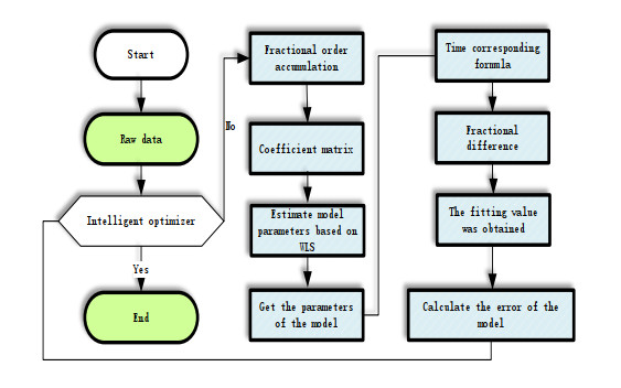
The fractional grey model is an effective tool for modeling small samples of data. Due to its essential characteristics of mathematical modeling, it has attracted considerable interest from scholars. A number of compelling methods have been proposed by many scholars in order to improve the accuracy and extend the scope of the application of the model. Examples include initial value optimization, order optimization, etc. The weighted least squares approach is used in this paper in order to enhance the model's accuracy. The first step in this study is to develop a novel fractional prediction model based on weighted least squares operators. Thereafter, the accumulative order of the proposed model is determined, and the stability of the optimization algorithm is assessed. Lastly, three actual cases are presented to verify the validity of the model, and the error variance of the model is further explored. Based on the results, the proposed model is more accurate than the comparison models, and it can be applied to real-world situations.

| [1] |
J. L. Deng, Control problems of grey systems, Syst. Control Lett., 1 (1982), 288–294. https://doi.org/10.1016/S0167-6911(82)80025-X doi: 10.1016/S0167-6911(82)80025-X

|
| [2] | J. L. Deng, Introduction to grey system theory, J. Grey Syst., 1 (1989), 1–24. |
| [3] | C. Y. Kung, C. P. Chang, Application of grey prediction model on China automobile industry, J. Grey Syst., 16 (2004), 147–154. |
| [4] |
X. Feng, S. Zhang, Measles trends dynamic forecasting model based on grey system theory, Manag. Sci. Eng., 6 (2012), 71–74. https://doi.org/10.3968/J.MSE.1913035X20120604.ZRXZ2 doi: 10.3968/J.MSE.1913035X20120604.ZRXZ2
|
| [5] | C. Wang, D. Zuo, G. Hong, Application of grey system theory to the determination of the dominant infectious diseases and the forecasting of the epidemic conditions, Anhui J. Preventive Med., 17 (2011), 180–183. |
| [6] | X. Li, Y. Dang, J. Zhao, An optimization method of estimating parameters in GM (1, 1) model, In: 2009 IEEE International Conference on Grey Systems and Intelligent Services (GSIS 2009), Nanjing, China, 2009. https://doi.org/10.1109/GSIS.2009.5408272 |
| [7] |
C. C. Hsu, C. Y. Chen, Applications of improved grey prediction model for power demand forecasting, Energy Convers. Manage., 44 (2003), 2241–2249. https://doi.org/10.1016/S0196-8904(02)00248-0 Ma1 doi: 10.1016/S0196-8904(02)00248-0
|
| [8] | X. Ma, W. Wu, Y. Zhang, Improved GM(1, 1) model based on Simpson formula and its applications, 2019. https://doi.org/10.48550/arXiv.1908.03493 |
| [9] |
S. Mao, Q. He, X. Xiao, C. Rao, Study of the correlation between oil price and exchange rate under the new state of the economy, Sci. Iran., 26 (2019), 2472–2483. http://dx.doi.org/10.24200/SCI.2018.20448 doi: 10.24200/SCI.2018.20448
|
| [10] |
W. Wu, X. Ma, Y. Wang, W. Cai, B. Zeng, Predicting China's energy consumption using a novel grey Riccati model, Appl. Soft Comput., 95 (2020), 106555. https://doi.org/10.1016/j.asoc.2020.106555 doi: 10.1016/j.asoc.2020.106555
|
| [11] |
J. Wang, P. Du, H. Lu, W. Yang, T. Niu, An improved grey model optimized by multi-objective ant lion optimization algorithm for annual electricity consumption forecasting, Appl. Soft Comput., 72 (2018), 321–337. https://doi.org/10.1016/j.asoc.2018.07.022 doi: 10.1016/j.asoc.2018.07.022
|
| [12] |
W. Z. Wu, T. Zhang, C. Zheng, A novel optimized nonlinear grey Bernoulli model for forecasting China's GDP, Complexity, 2019 (2019), 1–10. https://doi.org/10.1155/2019/1731262 doi: 10.1155/2019/1731262
|
| [13] |
W. Wu, X. Ma, B. Zeng, W. Lv, Y. Wang, W. Li, A novel Grey Bernoulli model for short-term natural gas consumption forecasting, Appl. Math. Model., 84 (2020), 393–404. https://doi.org/10.1016/j.apm.2020.04.006 doi: 10.1016/j.apm.2020.04.006
|
| [14] |
W. Wu, X. Ma, Y. Wang, W. Cai, B. Zeng, Predicting primary energy consumption using NDGM (1, 1, k, c) model with Simpson formula, Sci. Iran., 28 (2019), 3379–3395. https://doi.org/10.24200/SCI.2019.51218.2067 doi: 10.24200/SCI.2019.51218.2067
|
| [15] |
W. Zhou, Y. Cheng, S. Ding, L. Chen, R. Li, A grey seasonal least square support vector regression model for time series forecasting, ISA Trans., 114 (2020), 82–98. https://doi.org/10.1016/j.isatra.2020.12.024 doi: 10.1016/j.isatra.2020.12.024
|
| [16] |
L. Wu, S. Liu, L. Yao, S. Yan, D. Liu, Grey system model with the fractional order accumulation, Commun. Nonlinear Sci. Numer. Simul., 18 (2013), 1775–1785. https://doi.org/10.1016/j.cnsns.2012.11.017 doi: 10.1016/j.cnsns.2012.11.017
|
| [17] |
U. Şahin, Forecasting share of renewables in primary energy consumption and $CO_2$ emissions of China and the United States under Covid-19 pandemic using a novel fractional nonlinear grey model, Expert Syst. Appl., 209 (2022), 118429. https://doi.org/10.1016/j.eswa.2022.118429 doi: 10.1016/j.eswa.2022.118429
|
| [18] |
S. Yan, Q. Su, Z. Gong, X. Zeng, Fractional order time-delay multivariable discrete grey model for short-term online public opinion prediction, Expert Syst. Appl., 197 (2022), 116691. https://doi.org/10.1016/j.eswa.2022.116691 doi: 10.1016/j.eswa.2022.116691
|
| [19] |
S. Ding, Z. Tao, R. Li, X. Qin, A novel seasonal adaptive grey model with the data-restacking technique for monthly renewable energy consumption forecasting, Expert Syst. Appl., 208 (2022), 118115. https://doi.org/10.1016/j.eswa.2022.118115 doi: 10.1016/j.eswa.2022.118115
|
| [20] |
X. Ma, W. Wu, B. Zeng, Y. Wang, X. Wu, The conformable fractional grey system model, ISA Trans., 96 (2020), 255–271. https://doi.org/10.1016/j.isatra.2019.07.009 doi: 10.1016/j.isatra.2019.07.009
|
| [21] |
L. Chen, Z. Liu, N. Ma, Time-delayed polynomial grey system model with the fractional order accumulation, Mathe. Probl. Eng., 2018 (2018), 1–7. https://doi.org/10.1155/2018/3640625 doi: 10.1155/2018/3640625
|
| [22] |
H. Duan, G. R. Lei, K. Sha, Forecasting crude oil consumption in China using a grey prediction model with an optimal fractional-order accumulating operator, Complexity, 2018 (2018), 1–12. https://doi.org/10.1155/2018/3869619 doi: 10.1155/2018/3869619
|
| [23] |
W. Meng, D. Yang, H. Huang, Prediction of China's sulfur dioxide emissions by discrete grey model with fractional order generation operators, Complexity, 2018 (2018), 1–13. https://doi.org/10.1155/2018/8610679 doi: 10.1155/2018/8610679
|
| [24] |
W. Xie, C. Liu, W. Wu, W. Li, C. Liu, Continuous grey model with conformable fractional derivative, Chaos, Solitons Fract., 139 (2020), 110285. https://doi.org/10.1016/j.chaos.2020.110285 doi: 10.1016/j.chaos.2020.110285
|
| [25] |
W. Xie, W. Wu, C. Liu, J. Zhao, Forecasting annual electricity consumption in China by employing a conformable fractional grey model in opposite direction, Energy, 202 (2020), 117682. https://doi.org/10.1016/j.energy.2020.117682 doi: 10.1016/j.energy.2020.117682
|
| [26] | S. Mao, X. Xiao, M. Gao, X. Wang, Q. He, Nonlinear fractional order grey model of urban traffic flow short-term prediction, J. Grey Syst., 30 (2018), 1–17. |
| [27] |
W. Wu, X. Ma, Y. Zhang, W. Li, Y. Wang, A novel conformable fractional non-homogeneous grey model for forecasting carbon dioxide emissions of BRICS countries, Sci. Total Environ., 707 (2020), 135447. https://doi.org/10.1016/j.scitotenv.2019.135447 doi: 10.1016/j.scitotenv.2019.135447
|
| [28] |
W. Wu, X. Ma, B. Zeng, Y. Wang, W. Cai, Forecasting short-term renewable energy consumption of China using a novel fractional nonlinear grey Bernoulli model, Renew. Energy, 140 (2019), 70–87. https://doi.org/10.1016/j.renene.2019.03.006 doi: 10.1016/j.renene.2019.03.006
|
| [29] |
P. Gao, J. Zhan, J. Liu, Fractional-order accumulative linear time-varying parameters discrete grey forecasting model, Math. Probl. Eng., 2019 (2019), 1–12. https://doi.org/10.1155/2019/6343298 doi: 10.1155/2019/6343298
|
| [30] |
L. Wu, H. Zhao, Using FGM(1, 1) model to predict the number of the lightly polluted day in Jing-Jin-Ji region of China, Atmos. Pollut. Res., 10 (2019), 552–555. https://doi.org/10.1016/j.apr.2018.10.004 doi: 10.1016/j.apr.2018.10.004
|
| [31] |
L. Wu, N. Li, T. Zhao, Using the seasonal FGM(1, 1) model to predict the air quality indicators in Xingtai and Handan, Environ. Sci. Pollut. Res., 26 (2019), 14683–14688. https://doi.org/10.1007/s11356-019-04715-z doi: 10.1007/s11356-019-04715-z
|
| [32] |
W. Xie, C. Liu, W. Wu, The fractional non-equidistant grey opposite-direction model with time-varying characteristics, Soft Comput., 24 (2020), 6603–6612. https://doi.org/10.1007/s00500-020-04799-7 doi: 10.1007/s00500-020-04799-7
|
| [33] |
W. Xie, W. Wu, T. Zhang, Q. Li, An optimized conformable fractional non-homogeneous gray model and its application, Commun. Stat.-Simul. Comput., 51 (2022), 5988–6003. https://doi.org/10.1080/03610918.2020.1788588 doi: 10.1080/03610918.2020.1788588
|
| [34] |
F. Liu, W. Guo, R. Liu, J. Liu, Improved load forecasting model based on two-stage optimization of gray model with fractional order accumulation and Markov chain, Commun. Stat.-Theory Methods, 50 (2021), 2659–2673. https://doi.org/10.1080/03610926.2019.1674873 doi: 10.1080/03610926.2019.1674873
|
| [35] |
Y. Kang, S. Mao, Y. Zhong, H. Zhu, Fractional derivative multivariable grey model for nonstationary sequence and its application, J. Syst. Eng. Electron., 31 (2020), 1009–1018. https://doi.org/10.23919/JSEE.2020.000075 doi: 10.23919/JSEE.2020.000075
|
| [36] |
W. Wu, X. Ma, Y. Zhang, Y. Wang, X. Wu, Analysis of novel FAGM(1, 1, $t^\alpha$) model to forecast health expenditure of China, Grey Syst.: Theory Appl., 9 (2019), 232–250. https://doi.org/10.1108/GS-11-2018-0053 doi: 10.1108/GS-11-2018-0053
|
| [37] |
W. Wu, X. Ma, Y. Wang, Y. Zhang, B. Zeng, Research on a novel fractional GM($\alpha, n$) model and its applications, Grey Syst.: Theory Appl., 9 (2019), 356–373. https://doi.org/10.1108/GS-11-2018-0052 doi: 10.1108/GS-11-2018-0052
|
| [38] |
L. Liu, L. Wu, Forecasting the renewable energy consumption of the European countries by an adjacent non-homogeneous grey model, Appl. Math. Model., 89 (2021), 1932–1948. https://doi.org/10.1016/j.apm.2020.08.080 doi: 10.1016/j.apm.2020.08.080
|
| [39] |
Y. Yuan, H. Zhao, X. Yuan, L. Chen, X. Lei, Application of fractional order-based grey power model in water consumption prediction, Environ. Earth Sci., 78 (2019), 1–8. https://doi.org/10.1007/s12665-019-8257-5 doi: 10.1007/s12665-019-8257-5
|
| [40] |
Y. Kang, S. Mao, Y. Zhang, Fractional time-varying grey traffic flow model based on viscoelastic fluid and its application, Transport. Res. Part B: Meth., 157 (2022), 149–174. https://doi.org/10.1016/j.trb.2022.01.007 doi: 10.1016/j.trb.2022.01.007
|
| [41] |
S. Mao, Y. Zhang, Y. Kang, Y. Mao, Coopetition analysis in industry upgrade and urban expansion based on fractional derivative gray Lotka-Volterra model, Soft Comput., 15 (2021), 11485–11507. https://doi.org/10.1007/s00500-021-05878-z doi: 10.1007/s00500-021-05878-z
|
| [42] |
Y. Kang, S. Mao, Y. Zhang, Variable order fractional grey model and its application, Appl. Math. Model., 97 (2021), 619–635. https://doi.org/10.1016/j.apm.2021.03.059 doi: 10.1016/j.apm.2021.03.059
|
| [43] |
Y. Chen, L. Wu, L. Liu, Z. Kai, Fractional Hausdorff grey model and its properties, Chaos, Solitons Fract., 138 (2020), 109915. https://doi.org/10.1016/j.chaos.2020.109915 doi: 10.1016/j.chaos.2020.109915
|


Figures(8) / Tables(6)

Caixia Liu, Wanli Xie. An optimized fractional grey model based on weighted least squares and its application[J]. AIMS Mathematics, 2023, 8(2): 3949-3968. doi: 10.3934/math.2023198


 DownLoad: