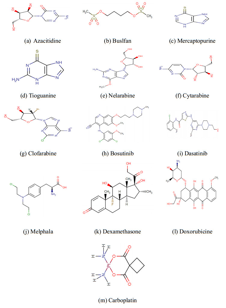
A topological index is a real number obtained from the chemical graph structure. It can predict the physicochemical and biological properties of many anticancer medicines like blood, breast and skin cancer. This can be done through degree-based topological indices.. In this article, the drugs, azacitidine, buslfan, mercaptopurine, tioguanine, nelarabine, etc. which are used in order to cure blood cancer are discussed and the purpose of the QSPR study is to determine the mathematical relation between the properties under investigation (eg, boiling point, flash point etc.) and different descriptors related to molecular structure of the drugs. It is found that topological indices (TIs) applied on said drugs have a good correlation with physicochemical properties in this context.
Citation: Sumiya Nasir, Nadeem ul Hassan Awan, Fozia Bashir Farooq, Saima Parveen. Topological indices of novel drugs used in blood cancer treatment and its QSPR modeling[J]. AIMS Mathematics, 2022, 7(7): 11829-11850. doi: 10.3934/math.2022660
A topological index is a real number obtained from the chemical graph structure. It can predict the physicochemical and biological properties of many anticancer medicines like blood, breast and skin cancer. This can be done through degree-based topological indices.. In this article, the drugs, azacitidine, buslfan, mercaptopurine, tioguanine, nelarabine, etc. which are used in order to cure blood cancer are discussed and the purpose of the QSPR study is to determine the mathematical relation between the properties under investigation (eg, boiling point, flash point etc.) and different descriptors related to molecular structure of the drugs. It is found that topological indices (TIs) applied on said drugs have a good correlation with physicochemical properties in this context.

| [1] |
B. Figuerola, C. Avila, The phylum bryozoa as a promising source of anticancer drugs, Mar. Drugs, 17 (2019), 477. https://doi.org/10.3390/md17080477 doi: 10.3390/md17080477

|
| [2] |
G. Genovese, A. K. Kähler, R. E. Handsaker, J. Lindberg, S. A. Rose, S. F. Bakhoum, et al., Clonal hematopoiesis and blood-cancer risk inferred from blood DNA sequence, New Eng. J. Med., 371 (2014), 2477-2487. https://doi.org/10.1056/NEJMoa1409405 doi: 10.1056/NEJMoa1409405
|
| [3] |
T. Terwilliger, M. J. B. C. J. Abdul-Hay, Acute lymphoblastic leukemia: A comprehensive review and 2017 update, Blood Cancer J., 7 (2017), e577-e577. https://doi.org/10.1038/bcj.2017.53 doi: 10.1038/bcj.2017.53
|
| [4] |
A. Aslam, Y. Bashir, S. Ahmad, W. Gao, On topological indices of certain dendrimer structures, Z. Naturforsch., 72 (2017), 559-566. https://doi.org/10.1515/zna-2017-0081 doi: 10.1515/zna-2017-0081
|
| [5] |
S. M. Hosamani, D. Perigidad, S. Jamagoud, Y. Maled, S. Gavade, QSPR anlysis of certain degree based topological indices, J. Statis. Appl. Prob., 6 (2017), 1-11. https://doi.org/10.18576/jsap/060211 doi: 10.18576/jsap/060211
|
| [6] | M. Randic, Comparative structure-property studies: regressions using a single descriptor, Croat. Chem. Acta, 66 (1993), 289-312. |
| [7] | M. Randic, Quantitative structure-propert relationship: boiling points and planar benzenoids, New J. Chem., 20 (1996) 1001-1009. |
| [8] |
M. C. Shanmukha, N. S. Basavarajappa, K. N. Anilkumar, Predicting physico-chemical properties of octane isomers using QSPR approach, Malaya J. Math., 8 (2020) 104-116. https://doi.org/10.26637/MJM0801/0018 doi: 10.26637/MJM0801/0018
|
| [9] |
S. Hayat, M. Imran, J. Liu, Correlation between the Estrada index and Q-electronic energies for benzenoid hydrocarbons with applica-tions to boron nanotubes, Int. J. Quant. Chem., 2019. https://doi.org/10.1002/qua.26016 doi: 10.1002/qua.26016
|
| [10] |
A. Aslam, S. Ahmad, W. Gao, On topological indices of boron triangular nanotubes, Z. Naturforsch., 72 (2017), 711-716. https://doi.org/10.1515/zna-2017-0135 doi: 10.1515/zna-2017-0135
|
| [11] |
S. Hayat, S. Wang, J. Liu, Valency-based topological descrip-tors of chemical networks and their applications, Appl. Math. Model., 2018. https://doi.org/10.1016/j.apm.2018.03.016 doi: 10.1016/j.apm.2018.03.016
|
| [12] | S. Hayat, M. Imran, J. Liu, An efficient computational technique for degree and distance based topological descriptors with applications, 2019. https://doi.org/10.1109/ACCESS.2019.2900500 |
| [13] | E. Estrada, L. Torres, L. Rodriguez, I. Gutman, An atom-bond connectivity index: Modeling the enthalpy of formation of alkanes, Indian J. Chem., 37A (1998), 849-855. |
| [14] |
T. Barbui, J. Thiele, H. Gisslinger, H. M. Kvasnicka, A. M. Vannucchi, P. Guglielmelli, et al., The 2016 WHO classification and diagnostic criteria for myeloproliferative neoplasms: document summary and in-depth discussion, Blood Cancer J., 8 (2018), 1-11. https://doi.org/10.1038/s41408-018-0054-y doi: 10.1038/s41408-018-0054-y
|
| [15] |
M. Randic, On Characterization of molecular branching, J. Am. Chem. Soc., 97 (1975), 6609-6615. https://doi.org/10.1021/ja00856a001 doi: 10.1021/ja00856a001
|
| [16] |
B. Zhou, N. Trinajstic, On general sum-connectivity index, J. Math. Chem., 47 (2010), 210-218. https://doi.org/10.1007/s10910-009-9542-4 doi: 10.1007/s10910-009-9542-4
|
| [17] |
D. Vukicevic, B. Furtula, Topological index based on the ratios of geometrical and arithmetical means of end-vertex degrees of edges, J. Math. Chem., 46 (2009), 1369-1376. https://doi.org/10.1007/s10910-009-9520-x doi: 10.1007/s10910-009-9520-x
|
| [18] |
M., Adnan, S. A. U. H. Bokhary, G. Abbas, T. Iqbal, Degree-based topological indices and QSPR analysis of antituberculosis drugs, J. Chem., 2022, Article ID 5748626. https://doi.org/10.1155/2022/5748626 doi: 10.1155/2022/5748626
|
| [19] |
I. Gutman, Degree based topological indices, Croat. Chem. Acta, 86 (2013), 351-361. https://doi.org/10.5562/cca2294 doi: 10.5562/cca2294
|
| [20] | S. Fajtlowicz, On conjectures of grafitti Ⅱ, Congr. Numerantium, 60 (1987), 189-197. |
| [21] | G. H. Shirdel, H. RezaPour, A. M. Sayadi, The hyper-zagreb index of graph operations, Iran. J. Math. Chem., 4 (2013), 213-220. |
| [22] |
M. Imran, M. K. Siddiqui, A. Q. Baig, W. Khalid, H. Shaker, Topological properties of cellular neural networks, J. Intell. Fuzzy Syst., 37 (2019), 3605-3614. https://doi.org/10.3233/JIFS-181813 doi: 10.3233/JIFS-181813
|
| [23] |
B. Furtula, I. Gutman, A forgotton topological index, J. Math. Chem., 53 (2015), 213-220. https://doi.org/10.1007/s10910-015-0480-z doi: 10.1007/s10910-015-0480-z
|
| [24] |
W. Gao, W. Wang, M. K. Jamil, M. R. FArhani, Electron energy studing of moleculer structurevia forgotten topological index computation, J. Chem., 2016. https://doi.org/10.1155/2016/1053183 doi: 10.1155/2016/1053183
|
| [25] | I. B. M. Corp, Released. IBM SPSS Statistics for Windows, Version 24.0 (Armonk, NY: IBM Corp., 2016). |
| [26] |
J. Liu, M. Arockiaraj, M. Arulperumjothi, S. Prabhu, Distance based and Bond additive topological indices of certain repurposed antiviral drug compounds tested for treating COVID- 19, Int. J. Quantum Chem., 121 (2021), e26617. https://doi.org/10.1002/qua.26617 doi: 10.1002/qua.26617
|
| [27] |
S. Prabhu, G. Murugan, M. Arockiaraj, M. Arulperumjothi, V. Manimozhi, Molecular topological characterization of three classes of polycyclic aromatic hydrocarbons, J. Mol. Struct., 1229 (2021), 129501. https://doi.org/10.1016/j.molstruc.2020.129501 doi: 10.1016/j.molstruc.2020.129501
|
| [28] |
S. Prabhu, Y. S. Nisha, M. Arulperumjothi, D. Sagaya Rani Jeba, V. Manimozhi, On detour index of Cycloparaphenylene and polyphenylene molecular structures, Sci. Rep-UK, 2021. https://doi.org/10.1038/s41598-021-94765-6 doi: 10.1038/s41598-021-94765-6
|
| [29] |
Y. Chu, K. Julietraja, P. Venugopal, M. K. Siddiqui, S. Prabhu, Degree- and irregularity-based molecular descriptors for benzenoid systems, Eur. Phys. J. Plus, 136 (2021), 78. https://doi.org/10.1140/epjp/s13360-020-01033-z doi: 10.1140/epjp/s13360-020-01033-z
|

Figures(2) / Tables(18)

Sumiya Nasir, Nadeem ul Hassan Awan, Fozia Bashir Farooq, Saima Parveen. Topological indices of novel drugs used in blood cancer treatment and its QSPR modeling[J]. AIMS Mathematics, 2022, 7(7): 11829-11850. doi: 10.3934/math.2022660


 DownLoad: