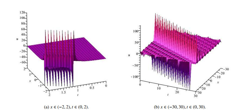
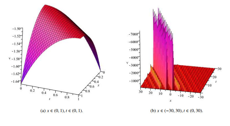
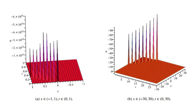
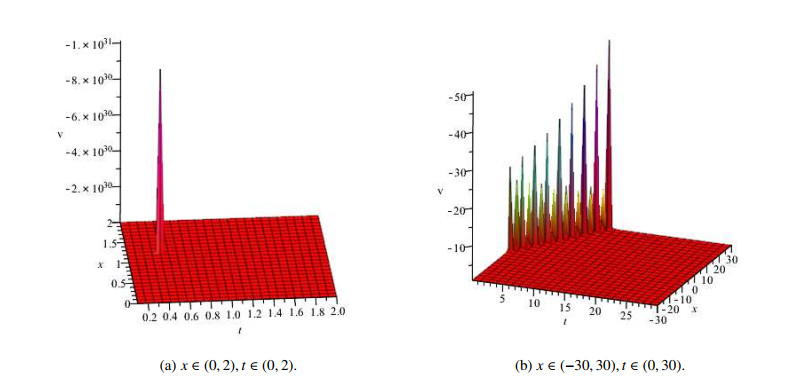
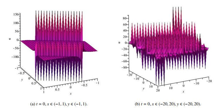
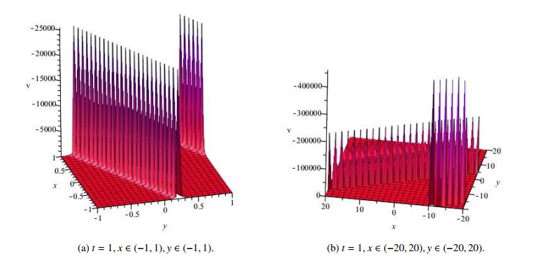
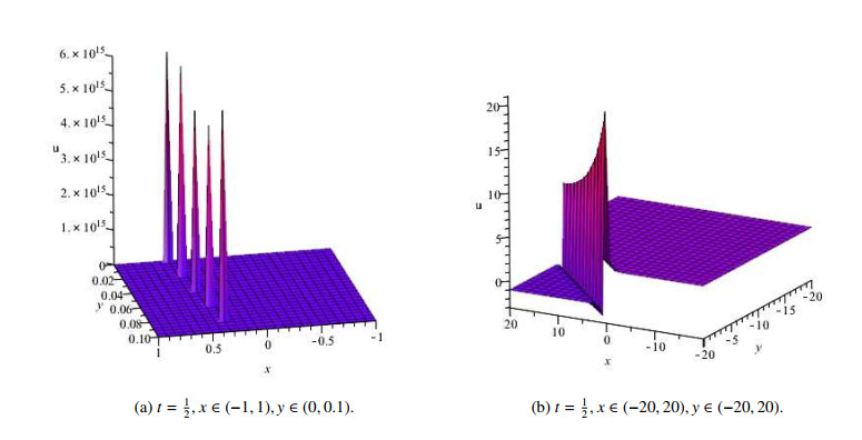
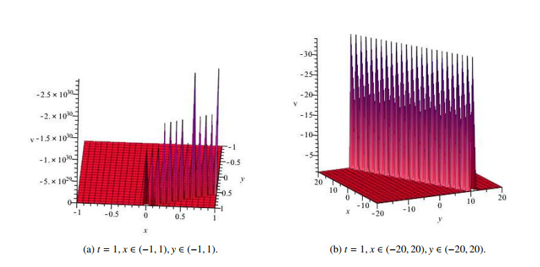
In this paper, eight groups of exact solutions for the (1+1)-dimensional and (2+1)-dimensional nonlinear dispersive long wave systems are found respectively via Feng's first integral method. It is shown that there are some similarities in the expressions of the solutions of (1+1)-dimensional and (2+1)-dimensional DLWEs, while there exist some differences in their dimensions and their physical significance. Finally, some graphs are presented to show these features, which also show the effectiveness of the proposed method.
Citation: Qiuci Lu, Songchuan Zhang, Hang Zheng. Exact solutions of a class of nonlinear dispersive long wave systems via Feng's first integral method[J]. AIMS Mathematics, 2021, 6(8): 7984-8000. doi: 10.3934/math.2021464
In this paper, eight groups of exact solutions for the (1+1)-dimensional and (2+1)-dimensional nonlinear dispersive long wave systems are found respectively via Feng's first integral method. It is shown that there are some similarities in the expressions of the solutions of (1+1)-dimensional and (2+1)-dimensional DLWEs, while there exist some differences in their dimensions and their physical significance. Finally, some graphs are presented to show these features, which also show the effectiveness of the proposed method.

| [1] |
X. Y. Gao, Y. J. Guo, W. R. Shan, Shallow water in an open sea or a wide channel: Auto- and non-auto-Backlund transformations with solitons for a generalized (2+1)-dimensional dispersive long-wave system, Chaos Solitons Fractals, 138 (2020), 109950. doi: 10.1016/j.chaos.2020.109950

|
| [2] |
H. Y. Zhang, Y. F. Zhang, Rational solutions and their interaction solutions for the (2+1)-dimensional dispersive long wave equation, Phys. Scr., 95 (2020), 045208. doi: 10.1088/1402-4896/ab5c89
|
| [3] | Y. Q. Zhou, Q. Liu, Bifurcation of travelling wave solutions for a (2+1)-dimensional nonlinear dispersive long wave equation, Appl. Math. Comput., 189 (2007), 970–979. |
| [4] |
Y. H. Tian, H. L. Chen, X. Q. Liu, Symmetry groups and new exact solutions of (2+1)-dimensional dispersive long-wave equations, Commun. Theor. Phys., 51 (2009), 781–784. doi: 10.1088/0253-6102/51/5/04
|
| [5] |
X. Y. Wen, New families of rational form variable separation solutions to (2+1)-dimensional dispersive long wave equations, Commun. Theor. Phys., 51 (2009), 789–793. doi: 10.1088/0253-6102/51/5/06
|
| [6] |
M. Boiti, J. J. P. Leon, F. Pempinelli, Spectral transform for a two spatial dimension extension of the dispersive long wave equation, Inverse Probl., 3 (1987), 371–387. doi: 10.1088/0266-5611/3/3/007
|
| [7] | S. Y. Lou, Similarity solutions of dispersive long wave equations in two space dimensions, Math. Meth. Appl. Sci., 18 (1995), 789–802. |
| [8] |
J. F. Zhang, Bácklund transformation and multisoliton-like solution of the (2+1)-dimensional dispersive long wave equations, Commun. Theor. Phys., 33 (2000), 577–582. doi: 10.1088/0253-6102/33/4/577
|
| [9] |
E. Yomba, Construction of new soliton-like solutions of the (2+1)-dimensional dispersive long wave equation, Chaos Solitons Fractals, 20 (2004), 1135–1139. doi: 10.1016/j.chaos.2003.09.026
|
| [10] |
A. Elgarayhi, New solitons and periodic wave solutions for the dispersive long wave equations, Phys. A, 361 (2006), 416–428. doi: 10.1016/j.physa.2005.05.103
|
| [11] | W. Zhu, Y. H. Xia, B. Zhang, Y. Bai, Exact traveling wave solutions and bifurcations of the time-fractional differential equations with applications, Int. J. Bifur. Chaos, 129 (2019), 1950041. |
| [12] | W. Zhu, Y. H. Xia, Y. Bai, Traveling wave solutions of the complex Ginzburg-Landau equation, Appl. Math. Comput., 382 (2020), 125342. |
| [13] | B. Zhang, Y. H. Xia, W. Zhu, Y. Bai, Explicit exact traveling wave solutions and bifurcations of the generalized combined double sinh-cosh-Gordon equation, Appl. Math. Comput., 363 (2019), 124576. |
| [14] |
B. Zhang, W. Zhu, Y. H. Xia, Y. Bai, A unified analysis of exact traveling wave solutions for the fractional-order and integer-order Biswas-Milovic equation: via bifurcation theory of dynamical system, Qual. Theory Dyn. Syst., 19 (2020), 11. doi: 10.1007/s12346-020-00352-x
|
| [15] |
K. Hosseini, P. Gholamin, Feng's first integral method for analytic treatment of two higher dimensional nonlinear partial differential equations, Differ. Equations Dyn. Syst., 23 (2015), 317–-325. doi: 10.1007/s12591-014-0222-x
|
| [16] |
Z. S. Feng, The first-integral method to study the Burgers-Korteweg-de Vries equation, J. Phys. A: Math. Gen., 35 (2002), 343–349. doi: 10.1088/0305-4470/35/2/312
|
| [17] |
Z. S. Feng, X. H. Wang, The first integral method to the two-dimensional Burgers-Korteweg-de Vries equation, Phys. Lett. A, 308 (2003), 173–178. doi: 10.1016/S0375-9601(03)00016-1
|
| [18] |
Z. Feng, S. Z. Zheng, D. Y. Gao, Traveling wave solutions to a reaction-diffusion equation, Z. Angew. Math. Phys., 60 (2009), 756–773. doi: 10.1007/s00033-008-8092-0
|
| [19] |
K. R. Raslan, The first integral method for solving some important nonlinear partial differential equations, Nonlinear Dyn., 53 (2008), 281–286. doi: 10.1007/s11071-007-9262-x
|
| [20] |
F. Tascan, A. Bekir, M. Koparan, Travelling wave solutions of nonlinear evolution equations by using the first integral method, Commun. Nonlinear Sci. Numer. Simul., 14 (2009), 1810–1815. doi: 10.1016/j.cnsns.2008.07.009
|
| [21] |
S. Abbasbandy, A. Shirzadi, The first integral method for modified Benjamin-Bona-Mahony equation, Commun. Nonlinear Sci. Numer. Simul., 15 (2010), 1759–1764. doi: 10.1016/j.cnsns.2009.08.003
|
| [22] |
K. Hosseini, R. Ansari, P. P. Gholamin, Exact solutions of some nonlinear systems of partial differential equations by using the first integral method, J. Math. Anal. Appl., 387 (2012), 807–814. doi: 10.1016/j.jmaa.2011.09.044
|
| [23] | M. F. El-Sabbagh, S. I. El-Ganaini, Travelling wave solutions of some important nonlinear systems using the first integral method, Adv. Studies Theor. Phys., 6 (2012), 831–842. |
| [24] | N. Bourbaki, Commutative algebra, Addison-Wesley, Paris, 1972. |
Figures(8)

Qiuci Lu, Songchuan Zhang, Hang Zheng. Exact solutions of a class of nonlinear dispersive long wave systems via Feng's first integral method[J]. AIMS Mathematics, 2021, 6(8): 7984-8000. doi: 10.3934/math.2021464


 DownLoad: