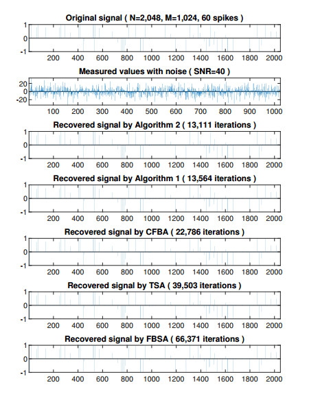
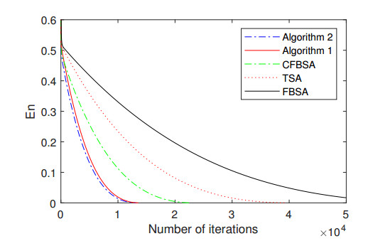
In this work, we introduce two modified Tseng's splitting algorithms with a new non-monotone adaptive step size for solving monotone inclusion problem in the framework of Banach spaces. Under some mild assumptions, we establish the weak and strong convergence results of the proposed algorithms. Moreover, we also apply our results to variational inequality problem, convex minimization problem and signal recovery, and provide several numerical experiments including comparisons with other related algorithms.
Citation: Jun Yang, Prasit Cholamjiak, Pongsakorn Sunthrayuth. Modified Tseng's splitting algorithms for the sum of two monotone operators in Banach spaces[J]. AIMS Mathematics, 2021, 6(5): 4873-4900. doi: 10.3934/math.2021286
In this work, we introduce two modified Tseng's splitting algorithms with a new non-monotone adaptive step size for solving monotone inclusion problem in the framework of Banach spaces. Under some mild assumptions, we establish the weak and strong convergence results of the proposed algorithms. Moreover, we also apply our results to variational inequality problem, convex minimization problem and signal recovery, and provide several numerical experiments including comparisons with other related algorithms.

| [1] |
H. A. Abass, C. Izuchukwu, O. T. Mewomo, Q. L. Dong, Strong convergence of an inertial forward-backward splitting method for accretive operators in real Banach space, Fixed Point Theory, 21 (2020), 397-412. doi: 10.24193/fpt-ro.2020.2.28

|
| [2] | R. P. Agarwal, D. O'Regan, D. R. Sahu, Fixed Point Theory for Lipschitzian-type Mappings with Applications, New York: Springer, 2009. |
| [3] | Y. I. Alber, Metric and generalized projection operators in Banach spaces: properties and applications, In: A. G. Kartsatos, Theory and Applications of Nonlinear Operator of Accretive and Monotone Type, New York: Marcel Dekker, (1996), 15-50. |
| [4] |
K. Ball, E. A. Carlen, E. H. Lieb, Sharp uniform convexity and smoothness inequalities for trace norms, Inventiones Math., 115 (1994), 463-482. doi: 10.1007/BF01231769
|
| [5] | V. Barbu, Nonlinear Semigroups and Differential Equations in Banach Spaces, Netherlands: Springer, 1976. |
| [6] | T. Bonesky, K. S. Kazimierski, P. Maass, F. Schöpfer, T. Schuster, Minimization of Tikhonov Functionals in Banach Spaces, Abstr. Appl. Anal., 2008 (2008), 192679. |
| [7] |
F. Browder, Nonlinear monotone operators and convex sets in Banach spaces, Bull. Am. Math. Soc., 71 (1965), 780-785. doi: 10.1090/S0002-9904-1965-11391-X
|
| [8] |
Y. Censor, A. Gibali, S. Reich, The subgradient extragradient method for solving variational inequalities in Hilbert space, J. Optim. Theory Appl., 148 (2011), 318-335. doi: 10.1007/s10957-010-9757-3
|
| [9] |
S. S. Chang, C. F. Wen, J. C. Yao, Generalized viscosity implicit rules for solving quasi-inclusion problems of accretive operators in Banach spaces, Optimization, 66 (2017), 1105-1117. doi: 10.1080/02331934.2017.1325888
|
| [10] |
S. S. Chang, C. F. Wen, J. C. Yao, A generalized forward-backward splitting method for solving a system of quasi variational inclusions in Banach spaces, RACSAM, 113 (2019), 729-747. doi: 10.1007/s13398-018-0511-2
|
| [11] |
G. H. Chen, R. T. Rockafellar, Convergence rates in forward-backward splitting, SIAM J. Optim., 7 (1997), 421-444. doi: 10.1137/S1052623495290179
|
| [12] |
P. Cholamjiak, A generalized forward-backward splitting method for solving quasi inclusion problems in Banach spaces, Numer. Algorithms, 71 (2016), 915-932. doi: 10.1007/s11075-015-0030-6
|
| [13] | P. Cholamjiak, N. Pholasa, S. Suantai, P. Sunthrayuth, The generalized viscosity explicit rules for solving variational inclusion problems in Banach spaces, Optimization, 2020. Available from: https://doi.org/10.1080/02331934.2020.1789131. |
| [14] | I. Cioranescu, Geometry of Banach Spaces, Duality Mappings and Nonlinear Problems, Dordrecht: Kluwer Academic, 1990. |
| [15] |
P. L. Combettes, V. R. Wajs, Signal recovery by proximal forward-backward splitting, Multiscale Model. Simul., 4 (2005), 1168-1200. doi: 10.1137/050626090
|
| [16] |
I. Daubechies, M. Defrise, C. De Mol, An iterative thresholding algorithm for linear inverse problems with a sparsity constraint, Commun. Pure Appl. Math., 57 (2004), 1413-1457. doi: 10.1002/cpa.20042
|
| [17] | J. Duchi, Y. Singer, Efficient online and batch learning using forward-backward splitting, J. Mach. Learn. Res., 10 (2009), 2899-2934. |
| [18] |
J. C. Dunn, Convexity, monotonicity, and gradient processes in Hilbert space, J. Math. Anal. Appl., 53 (1976), 145-158. doi: 10.1016/0022-247X(76)90152-9
|
| [19] |
A. Gibali, D. V. Thong, Tseng type methods for solving inclusion problems and its applications, Calcolo, 55 (2018), 49. doi: 10.1007/s10092-018-0292-1
|
| [20] |
O. G$\ddot{u}$ler, On the convergence of the proximal point algorithm for convex minimization, SIAM J. Control Optim., 29 (1991), 403-419. doi: 10.1137/0329022
|
| [21] | E. T. Hale, W. Yin, Y. Zhang, A fixed-point continuation method for $\ell_1$-regularized minimization with applications to compressed sensing, CAAM Technical Report TR07-07, 2007. |
| [22] | P. T. Harker, J. S. Pang, A damped-Newton method for the linear complementarity problem, In: G. Allgower, K. Georg, Computational Solution of Nonlinear Systems of Equations, AMS Lectures on Applied Mathematics, 26 (1990), 265-284. |
| [23] |
O. Hanner, On the uniform convexity of $L_p$ and $\ell_p$, Arkiv Matematik, 3 (1956), 239-244. doi: 10.1007/BF02589410
|
| [24] |
Hartman, G. Stampacchia, On some non linear elliptic differential functional equations, Acta Math., 115 (1966), 271-310. doi: 10.1007/BF02392210
|
| [25] |
H. Iiduka, W. Takahashi, Weak convergence of a projection algorithm for variational inequalities in a Banach space, J. Math. Anal. Appl., 339 (2008), 668-679. doi: 10.1016/j.jmaa.2007.07.019
|
| [26] |
C. Izuchukwu, C. C. Okeke, F. O. Isiogugu, Viscosity iterative technique for split variational inclusion problem and fixed point problem between Hilbert space and Banach space, J. Fixed Point Theory Appl., 20 (2018), 1-25. doi: 10.1007/s11784-018-0489-6
|
| [27] | C. C. Okeke, C. Izuchukwu, Strong convergence theorem for split feasibility problem and variational inclusion problem in real Banach spaces, Rend. Circolo Mat. Palermo, 2020. Available from: https://doi.org/10.1007/s12215-020-00508-3. |
| [28] | G. M. Korpelevich, The extragradient method for finding saddle points and other problems, Ekonomikai Mat. Metody, 12 (1976), 747-756. |
| [29] |
P. L. Lions, B. Mercier, Splitting algorithms for the sum of two nonlinear operators, SIAM J. Numer. Anal., 16 (1979), 964-979. doi: 10.1137/0716071
|
| [30] |
P. E. Maingé, Strong convergence of projected subgradient methods for nonsmooth and nonstrictly convex minimization, Set-Valued Anal., 16 (2008), 899-912. doi: 10.1007/s11228-008-0102-z
|
| [31] | J. Peypouquet, Convex Optimization in Normed Spaces: Theory, Methods and Examples, Springer Briefs in Optimization, 2015. |
| [32] | N. Pholasa, P. Cholamjiak, The regularization method for solving variational inclusion problems, Thai J. Math., 14 (2016), 369-381. |
| [33] |
H. Raguet, J. Fadili, G. Peyre, A generalized forward-backward splitting, SIAM J. Imaging Sci., 6 (2013), 1199-1226. doi: 10.1137/120872802
|
| [34] |
R. T. Rockafellar, Monotone operators and the proximal point algorithm, SIAM J. Control Optim., 14 (1976), 877-898. doi: 10.1137/0314056
|
| [35] |
R. T. Rockafellar, On the maximal monotonicity of subdifferential mappings, Pac. J. Math., 33 (1970), 209-216. doi: 10.2140/pjm.1970.33.209
|
| [36] |
R. T. Rockafellar, On the maximality of sums of nonlinear monotone operators, Trans. Amer. Math. Soc., 149 (1970), 75-88. doi: 10.1090/S0002-9947-1970-0282272-5
|
| [37] |
Y. Shehu, Convergence results of forward-backward algorithms for sum of monotone operators in Banach spaces, Results Math., 74 (2019), 138. doi: 10.1007/s00025-019-1061-4
|
| [38] |
Y. Shehu, G. Cai, Strong convergence result of forward-backward splitting methods for accretive operators in banach spaces with applications, RACSAM, 112 (2018), 71. doi: 10.1007/s13398-016-0366-3
|
| [39] | W. Takahashi, Nonlinear Functional Analysis, Yokohama: Yokohama Publishers, 2000. |
| [40] | S. Takahashi, W. Takahashi, Split common null point problem and shrinking projection method for generalized resolvents in two Banach spaces, J. Nonlinear Convex Anal., 17 (2016), 2171-2182. |
| [41] |
W. Takahashi, N. C. Wong, J. C. Yao, Two generalized strong convergence theorems of Halpern's type in Hilbert spaces and applications, Taiwan. J. Math., 16 (2012), 1151-1172. doi: 10.11650/twjm/1500406684
|
| [42] |
K. K. Tan, H. K. Xu, Approximating fixed points of nonexpansive mappings by the Ishikawa iteration process, J. Math. Anal. Appl., 178 (1993), 301-308. doi: 10.1006/jmaa.1993.1309
|
| [43] |
D. V. Thong, P. Cholamjiak, Strong convergence of a forward-backward splitting method with a new step size for solving monotone inclusions, Comput. Appl. Math., 38 (2019), 94. doi: 10.1007/s40314-019-0855-z
|
| [44] | R. Tibshirani, Regression shrinkage and selection via the lasso, J. Royal Statist. Soc., 58 (1996), 267-288. Available from: https://doi.org/10.1111/j.2517-6161.1996.tb02080.x. |
| [45] |
P. Tseng, A modified forward-backward splitting method for maximal monotone mappings, SIAM J. Control Optim., 38 (2000), 431-446. doi: 10.1137/S0363012998338806
|
| [46] |
Y. Wang, F. Wang, Strong convergence of the forward-backward splitting method with multiple parameters in Hilbert spaces, Optimization, 67 (2018), 493-505. doi: 10.1080/02331934.2017.1411485
|
| [47] |
H. K. Xu, Inequalities in Banach spaces with applications, Nonlinear Anal., 16 (1991), 1127-1138. doi: 10.1016/0362-546X(91)90200-K
|
| [48] |
H. K. Xu, Iterative algorithms for nonlinear operators, J. London Math. Soc., 66 (2002), 240-256. doi: 10.1112/S0024610702003332
|
| [49] |
Z. B. Xu, G. F. Roach, Characteristic inequalities of uniformly convex and uniformly smooth Banach spaces, J. Math. Anal. Appl., 157 (1991), 189-210. doi: 10.1016/0022-247X(91)90144-O
|
| [50] |
J. Yang, H. Liu, Strong convergence result for solving monotone variational inequalities in Hilbert space, Numer. Algorithms, 80 (2019), 741-752. doi: 10.1007/s11075-018-0504-4
|
| [51] |
J. Yang, H. Liu, G. Li, Convergence of a subgradient extragradient algorithm for solving monotone variational inequalities, Numer. Algorithms, 84 (2020), 389-405. doi: 10.1007/s11075-019-00759-x
|
Figures(6) / Tables(3)

Jun Yang, Prasit Cholamjiak, Pongsakorn Sunthrayuth. Modified Tseng's splitting algorithms for the sum of two monotone operators in Banach spaces[J]. AIMS Mathematics, 2021, 6(5): 4873-4900. doi: 10.3934/math.2021286


 DownLoad: