Processing math: 62%
Research article

On the theory of fractional terminal value problem with ψ-Hilfer fractional derivative

  • Received: 30 December 2019 Accepted: 12 May 2020 Published: 03 June 2020
  • MSC : 34A08, 34B15, 34A12, 47H10

  • In this paper, we prove the existence and uniqueness of solutions of a new class of boundary value problems of terminal type for ψ-Hilfer fractional differential equations. The technique used in the analysis relies on the Banach contraction principle and Krasnosleskii fixed point theorem. Moreover, we use generalized Gronwall inequality with singularity to establish uniqueness and continuous dependence of the δ-approximate solution. Finally, we demonstrate some examples to illustrate our main results.

    Citation: Mohammed A. Almalahi, Mohammed S. Abdo, Satish K. Panchal. On the theory of fractional terminal value problem with ψ-Hilfer fractional derivative[J]. AIMS Mathematics, 2020, 5(5): 4889-4908. doi: 10.3934/math.2020312

    Related Papers:

    [1] Abdelkrim Salim, Sabri T. M. Thabet, Imed Kedim, Miguel Vivas-Cortez . On the nonlocal hybrid (k,φ)-Hilfer inverse problem with delay and anticipation. AIMS Mathematics, 2024, 9(8): 22859-22882. doi: 10.3934/math.20241112
    [2] Kangqun Zhang . Existence and uniqueness of positive solution of a nonlinear differential equation with higher order Erdélyi-Kober operators. AIMS Mathematics, 2024, 9(1): 1358-1372. doi: 10.3934/math.2024067
    [3] Dumitru Baleanu, Babak Shiri . Nonlinear higher order fractional terminal value problems. AIMS Mathematics, 2022, 7(5): 7489-7506. doi: 10.3934/math.2022420
    [4] Yujun Cui, Chunyu Liang, Yumei Zou . Existence and uniqueness of solutions for a class of fractional differential equation with lower-order derivative dependence. AIMS Mathematics, 2025, 10(2): 3797-3818. doi: 10.3934/math.2025176
    [5] Dumitru Baleanu, Babak Shiri . Generalized fractional differential equations for past dynamic. AIMS Mathematics, 2022, 7(8): 14394-14418. doi: 10.3934/math.2022793
    [6] Qi Wang, Chenxi Xie, Qianqian Deng, Yuting Hu . Controllability results of neutral Caputo fractional functional differential equations. AIMS Mathematics, 2023, 8(12): 30353-30373. doi: 10.3934/math.20231550
    [7] Jun Moon . The Pontryagin type maximum principle for Caputo fractional optimal control problems with terminal and running state constraints. AIMS Mathematics, 2025, 10(1): 884-920. doi: 10.3934/math.2025042
    [8] Wei Zhang, Jifeng Zhang, Jinbo Ni . New Lyapunov-type inequalities for fractional multi-point boundary value problems involving Hilfer-Katugampola fractional derivative. AIMS Mathematics, 2022, 7(1): 1074-1094. doi: 10.3934/math.2022064
    [9] Dehong Ji, Weigao Ge . A nonlocal boundary value problems for hybrid ϕ-Caputo fractional integro-differential equations. AIMS Mathematics, 2020, 5(6): 7175-7190. doi: 10.3934/math.2020459
    [10] Isra Al-Shbeil, Abdelkader Benali, Houari Bouzid, Najla Aloraini . Existence of solutions for multi-point nonlinear differential system equations of fractional orders with integral boundary conditions. AIMS Mathematics, 2022, 7(10): 18142-18157. doi: 10.3934/math.2022998
  • In this paper, we prove the existence and uniqueness of solutions of a new class of boundary value problems of terminal type for ψ-Hilfer fractional differential equations. The technique used in the analysis relies on the Banach contraction principle and Krasnosleskii fixed point theorem. Moreover, we use generalized Gronwall inequality with singularity to establish uniqueness and continuous dependence of the δ-approximate solution. Finally, we demonstrate some examples to illustrate our main results.


    In the recent years, scientific community renders more attention on fractional differential equations, since their are effective tools in modeling many phenomena in applied sciences and engineering application such as acoustic control, rheology, polymer physics, porous media, medicine, electrochemistry, proteins, electromagnetics, economics, astrophysics, chemical engineering, signal processing, optics, chaotic dynamics, statistical physics and so on for more details, see [1,2,3,4]. Since boundary value problems of fractional differential equations represent an important class of applied analysis, therefore the said area was given more importance, see [5,6,7,8,9,10] and references therein.

    Terminal value problems for differential equation nowadays play an essential part in the modeling of numerous phenomena in physical science, engineering, and so forth. Also, it arise naturally in the simulation of techniques that are watched at a later point, eventually after the methodology has started.

    Existence theory for classical terminal value problems have been investigated by several researchers [11,12,13,14,15,16,17,18,19,20,21,22]. It is well known [23] that the comparison principle for initial value problems of ordinary differential equations is a very useful tool in the study of qualitative and quantitative theory. Recently, attempts have been made to study the corresponding comparison principle for terminal value problems (TVP) [24]. Benchohra et. al. [14], studied the existence results and uniqueness of solutions for a class of boundary value problems of terminal type for fractional differential equations with the Hilfer–Katugampola fractional derivative by using different types of classical fixed point theory such as the Banach contraction principle and Krasnoselskii's fixed point theorem.

    Motivated by the above-mentioned works, the objective of this work is to study conditions for the existence and uniqueness of the solutions for terminal value problem for fractional differential equations of the type

    Dα,β;ψa+y(t)=f(t,y(t),Dα,β;ψa+y(t)),  t(a,T],a>0 (1.1)
    y(T)=wR, (1.2)

    where Dα,β;ψa+() is the ψ-Hilfer fractional derivative of order α(0,1), type β[0,1] and f:(a,T]×R×RR is a given function. Moreover, we study the uniqueness and continuous dependence of the δ-approximate solution by generalized Gronwall inequality. To our knowledge, no papers on terminal value problem for implicit fractional differential equations exist in the literature, in particular for those involving the ψ-Hilfer fractional derivative.

    The rest of the paper is organized as follows. In section 2, we present some necessary definitions and results which are used throughout this paper. In section 3, we study the existence and uniqueness results of ψ-Hilfer fractional differential equation with the terminal condition by using some fixed point theorems such as Banach and Krasnoselskii. In section 4, we study the δ-approximate solution of the problem (1.1), (1.2). Also, four examples are included to illustrate the applicability of the results obtained.

    In this section, we recall some notations, definitions of the fractional differential equation which are using throughout this paper. Let [a,T]R+ with (0<a<T<), and let C[a,T] be the Banach space of continuous function y:[a,T]R with the norm yC[a,T]=max{|y(t)|:atT}. The weighted space C1γ;ψ[a,T] of continuous function y is defined by [25]

    C1γ;ψ[a,T]={y:(a,T]R;[ψ(t)ψ(a)]1γy(t)C[a,T]}, 0γ<1

    Obviously, C1γ;ψ[a,T] is a Banach space endowed with the norm

    yc1γ;ψ=maxt[a,T]|[ψ(t)ψ(a)]1γy(t)|.

    Definition 2.1. [26] Let α>0, yL1[a,b] and ψC1[a,b] be an increasing function with ψ(t)0, for all t[a,b]. Then, the left-sided ψ-Riemann-Liouville fractional integral of a function y is defined by

    Iα,ψa+y(t)=1Γ(α)taψ(s)(ψ(t)ψ(s))α1y(s)ds,

    where Γ() is the Euler gamma function defined by Γ(α)=0sα1esds, α>0.

    Definition 2.2. [27] Let n1<α<n, ( n=[α]+1), and y,ψCn[a,b] be two functions with an increasing ψ and ψ(t)0, for all t[a,b]. Then, the left-sided ψ-Riemann-Liouville fractional (ψ-Caputo) derivative of a function y of order α is defined by

    Dα,ψa+y(t)=(1ψ(t)ddt)nInα,ψa+y(t),

    and

    CDα,ψa+y(t)=Inα,ψa+(1ψ(t)ddt)ny(t),

    respectively.

    Definition 2.3. [25] Let n1<α<n, ( nN), and y,ψCn[a,T] be two functions such that ψ is increasing and ψ(t)0, for all t[a,T]. Then, the left-sided ψ-Hilfer fractional derivative of a function y of order α and type 0β1 is defined by

    Dα,β,ψa+y(t)=Iβ(nα);ψa+(1ψ(t)ddt)nI(1β)(nα);ψa+y(t)=Iβ(nα);ψa+Dγ;ψa+y(t), (γ=α+nβαβ). (2.1)

    In this paper we consider the case n=1, because 0<α<1.

    Lemma 2.4. [2] Let α>0 and 0γ<1. Then Iα,ψa+ is bounded from C1γ;ψ[a,b] into C1γ;ψ[a,b].

    Now, we introduce the following spaces

    Cα,β1γ;ψ[a,T]={yC1γ;ψ[a,T],Dα,β;ψa+yC1γ;ψ[a,T]}, 0γ<1

    and

    Cγ1γ;ψ[a,T]={yC1γ;ψ[a,T],Dγ;ψa+yC1γ;ψ[a,T]}, 0γ<1. (2.2)

    Lemma 2.5. [25] Let γ=α+βαβ where α(0,1), β[0,1], and yCγ1γ;ψ[a,T]. Then

    Iγ;ψa+Dγ;ψa+y=Iα;ψa+Dα,β;ψa+y,

    and

    Dγ;ψa+Iα;ψa+y=Dβ(1α);ψa+y.

    Lemma 2.6. [25] Let α>0, 0γ<1 and yC1γ[a,T], β[0,1]. Then

    Dα,β,ψa+Iα,ψa+y(t)=y(t).

    Lemma 2.7. [2] Let t>a. Then for α0 and γ>0, we have

    Iα,ψa+[ψ(t)ψ(a)]γ1=Γ(γ)Γ(α+γ)(ψ(t)ψ(a))α+γ1, t>a.

    and

    Dα,ψa+[ψ(t)ψ(a)]α1=0, for α(0,1).

    Lemma 2.8. [25] Let γ=α+βαβ where α(0,1), β[0,1], yCγ1γ;ψ[a,T] and I1γ;ψa+yC11γ,ψ[a,T]. Then, we have

    Iγ;ψa+Dγ,ψa+y(t)=y(t)I1γ;ψa+y(a)Γ(γ)(ψ(t)ψ(a))γ1.

    Lemma 2.9. [25] Let α>0,0γ<α and yC1γ,ψ[a,T] (0<a<T<). If γ<α, then Iα;ψa+:C1γ,ψ[a,T]C1γ,ψ[a,T] is continuous on [a,T] and satisfies

    Iα;ψa+ y(a)=limta+Iα;ψa+y(t)=0.

    Theorem 2.10. [28] (Krasnoselskii fixed point theorem). Let M be closed, convex, bounded and nonempty subset of a Banach space X and A,B be two operators such that

    (1) Au+BvM for all u,vM.

    (2) A is compact and continuous.

    (3) B is contraction mapping.

    Then there exists zM such that z=Az+Bz.

    Theorem 2.11. [29] (Banach's fixed point theorem). Let X be a Banach space and M be a nonempty closed subset of X, then any contraction mapping T:MM has a unique fixed point.

    Lemma 2.12. [30] (Generalized Gronwall's Inequality Lemma) Let α>0 and x,y be two nonnegative function locally integrable on [a,b]. Assume that g is nonnegative and nondecreasing, and let ψC1[a,b] be an increasing function such that ψ(t)0 for all t[a,b]. If

    x(t)y(t)+g(t)taψ(s)(ψ(t)ψ(s))α1x(s)ds,  t[a,b],

    then

    x(t)y(t)+tan=1[g(t)Γ(α)]nΓ(nα)ψ(s)(ψ(t)ψ(s))nα1y(s)ds,  t[a,b].

    If y be a nondecreasing function on [a,b], then

    x(t)y(t)Eα{g(t)Γ(α)[ψ(t)ψ(a)]α},  t[a,b],

    where Eα() is the Mittag-Leffler function defined by

    Eα(z)=n=0znΓ(αn+1), zC.

    Theorem 3.1. Let γ=α+βαβ, where α(0,1) and β[0,1]. If  f:(a,T] R  is a function such that f()C1γ,ψ[a,T], then yCγ1γ,ψ(a,T] satisfies the following problem

    HDα,β;ψa+y(t)=f(t),t(a,T],a>0 (3.1)
    y(T)=wR (3.2)

    if and only if y satisfies the following integral equation

    y(t)=(ψ(T)ψ(a))1γ(ψ(t)ψ(a))1γ[w1Γ(α)Taψ(s)(ψ(T)ψ(s))α1f(s)ds]+1Γ(α)taψ(s)(ψ(t)ψ(s))α1f(s)ds. (3.3)

    Proof. First, let yCγ1γ,ψ(a,T] be a solution of the problem (3.1), (3.2). We prove that y is also a solution of Eq (3.3). From the definition of Cγ1γ,ψ(a,T], Lemma 2.4, and using the definition 2.3, we have

    I1γ,ψa+y(t)C1γ,ψ[a,T] and Dγ;ψa+y(t)=D1,ψI1γ,ψa+y(t).

    By the definition of the space Cn1γ,ψ[a,T], it follows that

    I1γ,ψa+y(t)C11γ,ψ[a,T]. (3.4)

    Using Lemma 2.8, with α=γ, we obtain

    Iγ;ψa+Dγ,ψa+y(t)=y(t)I1γ;ψa+y(a)Γ(γ)(ψ(t)ψ(a))γ1, t(a,T]. (3.5)

    Since yCγ1γ,ψ[a,T], and using Lemma 2.5 with Eq (3.1), we have

    Iγ;ψa+Dγ;ψa+y(t)=Iα;ψa+ Dα,β;ψa+y(t)=Iα;ψa+f(t). (3.6)

    Comparing Eqs (3.5) and (3.6), we see that

    y(t)=I1γ;ψa+y(a)Γ(γ)(ψ(t)ψ(a))γ1+Iα;ψa+f(t) (3.7)

    Using Eq (3.2), we get

    y(t)=(ψ(T)ψ(a))1γ(ψ(t)ψ(a))1γ[w1Γ(α)Taψ(s)(ψ(T)ψ(s))α1f(s)ds]+1Γ(α)taψ(s)(ψ(t)ψ(s))α1f(s)ds.

    Hence y(t) satisfies the problem (3.1), (3.2).

    Conversely, Let yCγ1γ,ψ[a,T] be a function satisfying Eq (3.3). We prove that y is also a solution of the problem (3.1), (3.2). Apply the operator Dγ;ψa+ on both sides of Eq (3.3). Then, from Lemmas 2.7 and 2.5, we have

    Dγ;ψa+y(t)=Dγ;ψa+Iα;ψa+f(t)=Dβ(1α);ψa+f(t) (3.8)

    From Eq (3.4), we have Dγ;ψa+yC1γ;ψ[a,T], and hence, Eq (3.8) implies

    Dγ;ψa+y(t)=D1,ψI1γ,ψa+f(t)=Dβ(1α);ψa+f(t)C1γ;ψ[a,T]. (3.9)

    As f(t)C1γ;ψ[a,T], and from Lemma 2.4, it follows that

    I1β(1α);ψa+fC11γ;ψ[a,T] (3.10)

    From Eqs (3.9) and (3.10) and the definition of the space Cn1γ;ψ(a,T], we get

    I1β(1α);ψa+fC11γ;ψ[a,T].

    Now, by applying operator Iβ(1α);ψa+ on both sides of Eq (3.9) and using Lemmas 2.9, 2.8, we have

    Iβ(1α);ψa+Dγ;ψa+y(t)=f(t)I1β(1α);ψa+f(a)Γ(β(1α))(ψ(t)ψ(a))β(1α)1=f(t). (3.11)

    From Eq (2.1), the Eq (3.11) reduces to

    HDα,β;ψa+y(t)=f(t).

    that is, Eq (3.1) holds.

    Before given our main results, the following conditions must be satisfied

    H1 f:(a,T]×R×RR is continuous function such that f(,x(),y())Cβ(1α)1γ;ψ for all x,yC1γ;ψ[a,T].

    H2 There exist two constants L>0 and M(0,1) such that

    |f(t,x1,y1)f(t,x2,y2)|L|x1x2|+M|y1y2|,

    for all x1,y1,x2,y2R and t(a,T].

    In the forthcoming theorem, by using the Banach fixed point theorem, we prove the unique solution of the problem (1.1), (1.2)

    Theorem 3.2. Assume that (H1) and (H2) hold. If

    [2LΓ(γ)(1M)Γ(α+γ)(ψ(T)ψ(a))α]<1, (3.12)

    then the problem (1.1), (1.2) has a unique solution in Cγ1γ;ψ[a,T]Cα,β1γ;ψ[a,T].

    Proof. In view of Theorem 3.1, the solution of the problem (1.1), (1.2) is given by

    y(t)=(ψ(T)ψ(a))1γ(ψ(t)ψ(a))1γ[w1Γ(α)Taψ(s)(ψ(T)ψ(s))α1Ky(s)ds]+1Γ(α)taψ(s)(ψ(t)ψ(s))α1Ky(s)ds, (3.13)

    where Ky(t)=f(t,y(t),Ky(t)). Consider the operator F:C1γ;ψ[a,T]C1γ;ψ[a,T] defined by

    Fy(t)=(ψ(T)ψ(a))1γ(ψ(t)ψ(a))1γ[w1Γ(α)Taψ(s)(ψ(T)ψ(s))α1Ky(s)ds]+1Γ(α)taψ(s)(ψ(t)ψ(s))α1Ky(s)ds, (3.14)

    by Lemma 2.4, we deduce that FyC1γ;ψ[a,T]. The proof will be given in two steps

    Step(1): We show that the operator F has a unique fixed point ˆy in C1γ;ψ[a,T]. Let y,yC1γ;ψ[a,T] and t(a,T]. Then, we have

    |Fy(t)Fy(t)|1Γ(α)(ψ(T)ψ(a))1γ(ψ(t)ψ(a))1γTaψ(s)(ψ(T)ψ(s))α1|Ky(s)Ky(s)|ds+1Γ(α)taψ(s)(ψ(t)ψ(s))α1|Ky(s)Ky(s)|ds,

    where Ky(s),Ky(s)C1γ;ψ[a,T] such that

    Ky(s)=f(s,y(s),Ky(s))
    Ky(s)=f(s,y(s),Ky(s)).

    By (H2), we have

    |Ky(s)Ky(s)|=|f(s,y(s),Ky(s))f(s,y(s),Ky(s))|L|y(s)y(s)|+M|Ky(s)Ky(s)|,

    which implies

    |Ky(s)Ky(s)|L1M|y(s)y(s)|. (3.15)

    Then for any t(a,T], we have

    |Fy(t)Fy(t)|L(1M)Γ(α)(ψ(T)ψ(a))1γ(ψ(t)ψ(a))1γTaψ(s)(ψ(T)ψ(s))α1|y(s)y(s)|ds+L(1M)Γ(α)taψ(s)(ψ(t)ψ(s))α1|y(s)y(s)|dsLyyC1γ,ψ[a,T](1M)Γ(α)(ψ(T)ψ(a))1γ(ψ(t)ψ(a))1γTaψ(s)(ψ(T)ψ(s))α1(ψ(s)ψ(0))γ1ds+LyyC1γ,ψ[a,T](1M)Γ(α)taψ(s)(ψ(t)ψ(s))α1(ψ(s)ψ(0))γ1ds.

    In view of Lemma 2.7, we obtain

    |Fy(t)Fy(t)|[LΓ(γ)yyC1γ,ψ[a,T](1M)Γ(α+γ)(ψ(T)ψ(a))α(ψ(t)ψ(a))1γ+LΓ(γ)yyC1γ,ψ[a,T](1M)Γ(α+γ)(ψ(t)ψ(a))α+γ1][2LΓ(γ)(1M)Γ(α+γ)(ψ(T)ψ(a))α](ψ(t)ψ(a))γ1yyC1γ,ψ[a,T].

    Hence

    |(ψ(t)ψ(a))1γ[Fy(t)Fy(t)]|[2LΓ(γ)(1M)Γ(α+γ)(ψ(T)ψ(a))α]yyC1γ,ψ[a,T],

    which implies that

    FyFyC1γ,ψ[2LΓ(γ)(1M)Γ(α+γ)(ψ(T)ψ(a))α]yyC1γ,ψ[a,T].

    Due to Eq (3.12), we deduce that the operator F is a contraction mapping. According to Banach's contraction principle, we conclude that F has a unique fixed point ˆyC1γ;ψ[a,T].

    Step(2): We show that such a fixed point ˆyC1γ;ψ[a,T] is actually in Cγ1γ;ψ(a,T]. Since ˆy is the unique fixed point of F in C1γ;ψ[a,T], then, for each t(a,T], we have

    ˆy(t)=(ψ(T)ψ(a))1γ(ψ(t)ψ(a))1γ[w1Γ(α)Taψ(s)(ψ(T)ψ(s))α1Kˆy(s)ds]+1Γ(α)taψ(s)(ψ(t)ψ(s))α1Kˆy(s)ds.

    Multiplying both sides of the last equation by Dγ,ψa+, using Lemmas 2.7 and 2.5, we have

    Dγ,ψa+ˆy(t)=Dγ,ψa+Iα;ψa+Kˆy(s)(t)=Dβ(1α);ψa+Kˆy(t),

    Since γα, by (H1), we have Dβ(1α);ψa+Kˆy(t)C1γ;ψ[a,T], and hence Dγ,ψa+ˆyC1γ;ψ[a,T]. It follows from definition of Cγ1γ;ψ[a,T] that ˆyCγ1γ;ψ[a,T]. As a consequence of the above steps, we conclude that the problem (1.1), (1.2) has a unique solution in Cγ1γ;ψ[a,T].

    We present now the second result, which is based on Krasnoselskii fixed point theorem.

    Theorem 3.3. Assume that (H1) and (H2) hold. Then the problem (1.1), (1.2) has at least one solution in Cγ1γ;ψ[a,T].

    Proof. Defined the closed, bounded, convex and nonempty set

    kξ={yC1γ;ψ[a,T]:y1γ;ψξ},

    with

    ξ(ψ(T)ψ(a))1γ[|w|+RΓ(γ)Γ(α+γ)(ψ(T)ψ(a))α+γ1].

    Set N=supt(a,T]|f(t,0,0)|. We split the operator F which defined by Eq (3.14) into two operators F1,F2 in kξ as following

    F1y(t)=(ψ(T)ψ(a))1γ(ψ(t)ψ(a))1γ[w1Γ(α)Taψ(s)(ψ(T)ψ(s))α1Ky(s)ds],

    and

    F2y(t)=1Γ(α)taψ(s)(ψ(t)ψ(s))α1Ky(s)ds.                                          

    Note that Fy(t)=F1y(t)+F2y(t). The proof will be divided into several steps as follows:

    Step(1):We show that F1y(t)+F2v(t)kξ for any y,vkξ.

    (ⅰ) For t(a,T] and ykξ, we have

    |(ψ(t)ψ(a))1γF1y(t)|(ψ(T)ψ(a))1γ[|w|+1Γ(α)Taψ(s)(ψ(T)ψ(s))α1|Ky(s)|ds](ψ(T)ψ(a))1γ[|w|+1Γ(α)Taψ(s)(ψ(T)ψ(s))α1(ψ(t)ψ(a))γ1                           |(ψ(t)ψ(a))1γKy(s)|ds]. (3.16)

    From (H2), we have

    |Ky(t)|=|f(t,y(t),Ky(t))|=|f(t,y(t),Ky(t))f(t,0,0)+f(t,0,0)||f(t,y(t),Ky(t))f(t,0,0)|+|f(t,0,0)|L|y(t)|+M|Ky(t)|+N.

    Multiplying both sides of the last inequality by (ψ(t)ψ(a))1γ, we get

    |(ψ(t)ψ(a))1γKy(t)|L|(ψ(t)ψ(a))1γy(t)|+(ψ(t)ψ(a))1γN+M|(ψ(t)ψ(a))1γKy(t)|Lξ+(ψ(T)ψ(a))1γN+M|(ψ(t)ψ(a))1γKy(t)|.

    Then, for each t(a,T], we have

    |(ψ(t)ψ(a))1γKy(t)|Lξ+(ψ(T)ψ(a))1γN1M:=R

    Thus, the Eq (3.16) and Lemma 2.7, imply that

    F1y1γ;ψ(ψ(T)ψ(a))1γ[|w|+RΓ(γ)Γ(α+γ)(ψ(T)ψ(a))α+γ1]. (3.17)

    (ⅱ) In a similar manner, for t(a,T], vkξ, we get

    F2v1γ;ψRΓ(γ)Γ(α+γ)(ψ(T)ψ(a))α+1γ. (3.18)

    Linking Eqs (3.17) and (3.18), for any y,vkξ, we obtain

    F1y+F2v1γ;ψmax{F1y1γ;ψ,F2v1γ;ψ}(ψ(T)ψ(a))1γ[|w|+RΓ(γ)Γ(α+γ)(ψ(T)ψ(a))α+γ1]ξ,

    which implies that F1y(t)+F2v(t)kξ.

    Step(2): We show that F1 is a contraction mapping. From Theorem 3.2, we have already proved that F is a contraction mapping and hence F1 is a contraction mapping too in kξ.

    Step(3): We show that F2 is a compact and continuous in kξ.

    The continuity of F2 follows from the continuity of f. Now, we need only to prove that F2 is compact (i.e F2 uniformly bounded and equicontinuous). From Eq (3.18), for any vkξ, we have

    F2v1γ;ψRΓ(γ)Γ(α+γ)(ψ(T)ψ(a))α+1γ.

    This means that F2 is uniformly bounded in kξ. Next, we show that F2 is equicontinuous in kξ. Let ykξ and t1,t2(a,T] such that t1<t2. Then, we have  

    |(ψ(t2)ψ(a))1γF2y(t2)(ψ(t1)ψ(a))1γF2y(t1)|=|(ψ(t2)ψ(a))1γΓ(α)t2aψ(s)(ψ(t2)ψ(s))α1Ky(s)ds(ψ(t1)ψ(a))1γΓ(α)t1aψ(s)(ψ(t1)ψ(s))α1Ky(s)ds|(ψ(t2)ψ(a))1γΓ(α)t2t1ψ(s)(ψ(t2)ψ(s))α1|Ky(s)|ds+1Γ(α)t1a|[ψ(s)(ψ(t2)ψ(a))1γ(ψ(t2)ψ(s))α1ψ(s)(ψ(t1)ψ(a))1γ(ψ(t1)ψ(s))α1]||Ky(s)|dsKy()C1γ,ψ(ψ(t2)ψ(a))1γΓ(γ)Γ(α+γ)(ψ(t2)ψ(t1))α+γ1+Ky()C1γ,ψΓ(α)t1a|[ψ(s)(ψ(t2)ψ(s))α1(ψ(t2)ψ(a))1γψ(s)(ψ(t1)ψ(s))α1(ψ(t1)ψ(a))1γ]|(ψ(s)ψ(a))γ1ds0    as  t2t1.

    This means that \mathcal{F}_{2} is equicontinuous in \mathcal{\Bbbk } _{\xi }. Hence \mathcal{F}_{2} is relatively compact on \mathcal{\Bbbk } _{\xi }. By Arzelá-Ascoli Theorem, we deduce that \mathcal{F}_{2} is compact on \mathcal{\Bbbk }_{\xi }. According to Theorem (2.10), we conclude that \mathcal{F} has at least a fixed

    point \widehat{y}\in C_{1-\gamma; \psi }\left[a, T\right] and by the same way of the proof of Theorem 3.2, we can easily show that \widehat{y} \in C_{1-\gamma; \psi }^{\gamma }\left[a, T\right]. Thus the problem (1.1), (1.2) has at least one solution in C_{1-\gamma; \psi }^{\gamma } \left[a, T\right] .

    Definition 4.1 A function y\in C_{1-\gamma, \psi }^{\gamma }\left[a, T \right] satisfying the \psi -Hilfer implicit fractional differential inequality

    \begin{equation} \left\Vert ^{H}D_{a^{+}}^{\alpha , \beta ;\psi }z(t)-f\left( t, z(t), ^{H}D_{a^{+}}^{\alpha , \beta ;\psi }z(t)\right) \right\Vert \leq \delta , t\in \left( a, T\right] , \end{equation} (4.1)

    and

    \begin{equation*} z(T) = w^{\ast }, \end{equation*}

    is called \delta -approximate solutions of \psi -Hilfer implicit fractional differential (1.1), (1.2)

    Theorem 4.2. Let f:\left(a, T\right] \times \mathbb{R} \times \mathbb{R} \rightarrow \mathbb{R} be a continuous function satisfies the condition (H _{2} ) for each t\in J and. Let z_{i}\in C_{1-\gamma, \psi }^{\gamma }\left(a, T\right], i = 1, 2, be a \delta -approximation solutions of the following \psi -Hilfer implicit fractional differential equation

    \begin{equation} \begin{array}{c} ^{H}D_{a^{+}}^{\alpha , \beta ;\psi }z_{i}(t) = f\left( t, z_{i}(t), ^{H}D_{a^{+}}^{\alpha , \beta ;\psi }z_{i}(t)\right) , ~~t\in \left( a, T\right] \\ z_{i}(T) = w_{i}^{\ast }. \end{array} , \end{equation} (4.2)

    Then

    \begin{eqnarray*} &&\left\Vert z_{1}-z_{2}\right\Vert _{C_{1-\gamma , \psi }} \\ &\leq &\Upsilon ^{-1}\left\{ \left( \delta _{1}+\delta _{2}\right) \left[ \frac{\left( \psi (t)-\psi (a)\right) ^{\alpha -\gamma +1}}{\Gamma (\alpha +1)}+\sum\limits_{n = 1}^{\infty }\left( \frac{L}{1-M}\right) ^{n}\frac{\left( \psi (t)-\psi (a)\right) ^{(n+1)\alpha -\gamma +1}}{\Gamma ((n+1)\alpha +1)} \right] \right. \\ &&\left. +\left\vert \left( w_{1}^{\ast }-w_{2}^{\ast }\right) \left( \psi (T)-\psi (a)\right) ^{1-\gamma }\right\vert \left[ 1+\sum\limits_{n = 1}^{ \infty }\left( \frac{L}{1-M}\right) ^{n}\frac{\Gamma (\gamma )}{\Gamma (n\alpha +\gamma )}(\psi (t)-\psi (a))^{n\alpha }\right] \right\} , \end{eqnarray*}

    where

    \begin{equation*} \Upsilon = \left\{ 1-\left( \psi (T)-\psi (a)\right) ^{\alpha }\frac{L}{1-M} \frac{\Gamma (\gamma )}{\Gamma (\alpha +\gamma )}\left[ 1+\sum \limits_{n = 1}^{\infty }\left( \frac{L}{1-M}\right) ^{n}\frac{\Gamma (\gamma ) }{\Gamma (n\alpha +\gamma )}(\psi (t)-\psi (a))^{n\alpha }\right] \right\} \end{equation*}

    Proof. Let z_{i}\in C_{1-\gamma, \psi }^{\gamma }\left(a, T\right], i = 1, 2, be an \delta -approximation solutions of the problem (4.2). Then, we have

    \begin{equation} \left\Vert ^{H}D_{a^{+}}^{\alpha , \beta ;\psi }z_{i}(t)-f\left( t, z_{i}(t), ^{H}D_{a^{+}}^{\alpha , \beta ;\psi }z_{i}(t)\right) \right\Vert \leq \delta _{i}, \ t\in \left( a, T\right] , i = 1, 2 \end{equation} (4.3)

    and

    \begin{equation*} z_{i}(T) = w_{i}^{\ast }. \end{equation*}

    Applying I_{a^{+}}^{\alpha, \psi } on both sides of the above inequality, and using lemma 2.8, we get

    \begin{eqnarray} &&\left. \left( \psi (t)-\psi (a)\right) ^{\alpha }\frac{\delta _{i}}{\Gamma (\alpha +1)}\geq \right. \\ &&\left\vert z_{i}(t)-w_{i}^{\ast }\frac{\left( \psi (T)-\psi (a)\right) ^{1-\gamma }}{(\psi (t)-\psi (a))^{1-\gamma }}+\frac{\left( \psi (T)-\psi (a)\right) ^{1-\gamma }}{(\psi (t)-\psi (a))^{1-\gamma }}\text{ } I_{a^{+}}^{\alpha , \psi }K_{z_{i}}(T)-\text{ }I_{a^{+}}^{\alpha , \psi }K_{z_{i}}(t)\right\vert \end{eqnarray}

    Using the fact \left\vert x\right\vert -\left\vert y\right\vert \leq \left\vert x-y\right\vert \leq \left\vert x\right\vert +\left\vert y\right\vert in the above inequality, we have

    \begin{eqnarray*} &&\left. \left( \psi (t)-\psi (a)\right) ^{\alpha }\frac{\delta _{1}+\delta _{2}}{\Gamma (\alpha +1)}\geq \right. \\ &&\left\vert z_{1}(t)-w_{1}^{\ast }\frac{\left( \psi (T)-\psi (a)\right) ^{1-\gamma }}{(\psi (t)-\psi (a))^{1-\gamma }}+\frac{\left( \psi (T)-\psi (a)\right) ^{1-\gamma }}{(\psi (t)-\psi (a))^{1-\gamma }}\text{ } I_{a^{+}}^{\alpha , \psi }K_{z_{1}}(T)-\text{ }I_{0^{+}}^{\alpha , \psi }K_{z_{1}}(t)\right\vert \\ &&+\left\vert z_{2}(t)-w_{2}^{\ast }\frac{\left( \psi (T)-\psi (a)\right) ^{1-\gamma }}{(\psi (t)-\psi (a))^{1-\gamma }}+\frac{\left( \psi (T)-\psi (a)\right) ^{1-\gamma }}{(\psi (t)-\psi (a))^{1-\gamma }}\text{ } I_{a^{+}}^{\alpha , \psi }K_{z_{2}}(T)-\text{ }I_{0^{+}}^{\alpha , \psi }K_{z_{2}}(t)\right\vert \\ &\geq &\left\vert \left[ z_{1}(t)-w_{1}^{\ast }\frac{\left( \psi (T)-\psi (a)\right) ^{1-\gamma }}{(\psi (t)-\psi (a))^{1-\gamma }}+\frac{\left( \psi (T)-\psi (a)\right) ^{1-\gamma }}{(\psi (t)-\psi (a))^{1-\gamma }}\text{ } I_{a^{+}}^{\alpha , \psi }K_{z_{1}}(T)-\text{ }I_{0^{+}}^{\alpha , \psi }K_{z_{1}}(t)\right] \right. \\ &&\left. -\left[ z_{2}(t)-w_{2}^{\ast }\frac{\left( \psi (T)-\psi (a)\right) ^{1-\gamma }}{(\psi (t)-\psi (a))^{1-\gamma }}+\frac{\left( \psi (T)-\psi (a)\right) ^{1-\gamma }}{(\psi (t)-\psi (a))^{1-\gamma }}\text{ } I_{a^{+}}^{\alpha , \psi }K_{z_{2}}(T)-\text{ }I_{a^{+}}^{\alpha , \psi }K_{z_{2}}(t)\right] \right\vert \\ &\geq &\left\vert \left( z_{1}(t)-z_{2}(t)\right) -\left( w_{1}^{\ast }-w_{2}^{\ast }\right) \frac{\left( \psi (T)-\psi (a)\right) ^{1-\gamma }}{ (\psi (t)-\psi (a))^{1-\gamma }}+\frac{\left( \psi (T)-\psi (a)\right) ^{1-\gamma }}{(\psi (t)-\psi (a))^{1-\gamma }}I_{a^{+}}^{\alpha , \psi }\left[ K_{z_{1}}(T)-K_{z_{2}}(T)\right] \right. \\ &&-\left. I_{a^{+}}^{\alpha , \psi }\left[ K_{z_{1}}(t)-K_{z_{2}}(t)\right] \right\vert \\ &\geq &\left\vert \left( z_{1}(t)-z_{2}(t)\right) \right\vert -\left\vert \left( w_{1}^{\ast }-w_{2}^{\ast }\right) \frac{\left( \psi (T)-\psi (a)\right) ^{1-\gamma }}{(\psi (t)-\psi (a))^{1-\gamma }}\right\vert +\left\vert \frac{\left( \psi (T)-\psi (a)\right) ^{1-\gamma }}{(\psi (t)-\psi (a))^{1-\gamma }}I_{a^{+}}^{\alpha , \psi }\left[ K_{z_{1}}(T)-K_{z_{2}}(T)\right] \right\vert \\ &&-\left\vert I_{a^{+}}^{\alpha , \psi }\left[ K_{z_{1}}(t)-K_{z_{2}}(t) \right] \right\vert \end{eqnarray*}

    In consequence, we have

    \begin{eqnarray*} &&\left\vert \left( z_{1}(t)-z_{2}(t)\right) \right\vert \\ &\leq &\left( \psi (t)-\psi (a)\right) ^{\alpha }\frac{\delta _{1}+\delta _{2}}{\Gamma (\alpha +1)}+\left\vert \left( w_{1}^{\ast }-w_{2}^{\ast }\right) \frac{\left( \psi (T)-\psi (a)\right) ^{1-\gamma }}{(\psi (t)-\psi (a))^{1-\gamma }}\right\vert \\ &&-\left\vert \frac{\left( \psi (T)-\psi (a)\right) ^{1-\gamma }}{(\psi (t)-\psi (a))^{1-\gamma }}I_{a^{+}}^{\alpha , \psi }\left[ K_{z_{1}}(T)-K_{z_{2}}(T)\right] \right\vert +\left\vert I_{a^{+}}^{\alpha , \psi }\left[ K_{z_{1}}(t)-K_{z_{2}}(t)\right] \right\vert \\ &\leq &\left( \psi (t)-\psi (a)\right) ^{\alpha }\frac{\delta _{1}+\delta _{2}}{\Gamma (\alpha +1)}+\left\vert \left( w_{1}^{\ast }-w_{2}^{\ast }\right) \frac{\left( \psi (T)-\psi (a)\right) ^{1-\gamma }}{(\psi (t)-\psi (a))^{1-\gamma }}\right\vert \\ &&+\frac{\left( \psi (T)-\psi (a)\right) ^{1-\gamma }}{(\psi (t)-\psi (a))^{1-\gamma }}\left\vert I_{a^{+}}^{\alpha , \psi }\left[ K_{z_{1}}(T)-K_{z_{2}}(T)\right] \right\vert +\left\vert I_{a^{+}}^{\alpha , \psi }\left[ K_{z_{1}}(t)-K_{z_{2}}(t)\right] \right\vert \\ &\leq &\left( \psi (t)-\psi (a)\right) ^{\alpha }\frac{\delta _{1}+\delta _{2}}{\Gamma (\alpha +1)}+\left\vert \left( w_{1}^{\ast }-w_{2}^{\ast }\right) \frac{\left( \psi (T)-\psi (a)\right) ^{1-\gamma }}{(\psi (t)-\psi (a))^{1-\gamma }}\right\vert \\ &&+\frac{\left( \psi (T)-\psi (a)\right) ^{1-\gamma }}{(\psi (t)-\psi (a))^{1-\gamma }}\frac{L}{1-M}\frac{1}{\Gamma (\alpha )}\int_{a}^{T}\psi ^{\prime }(s)\left( \psi (T)-\psi (s)\right) ^{\alpha -1}\left\vert z_{1}(s)-z_{2}(s)\right\vert ds \\ &&+\frac{1}{\Gamma (\alpha )}\int_{a}^{t}\psi ^{\prime }(s)\left( \psi (t)-\psi (s)\right) ^{\alpha -1}\left\vert y_{1}(s)-y_{2}(s)\right\vert ds \\ &\leq &\left( \psi (t)-\psi (a)\right) ^{\alpha }\frac{\delta _{1}+\delta _{2}}{\Gamma (\alpha +1)}+\left\vert \left( w_{1}^{\ast }-w_{2}^{\ast }\right) \frac{\left( \psi (T)-\psi (a)\right) ^{1-\gamma }}{(\psi (t)-\psi (a))^{1-\gamma }}\right\vert \\ &&+\frac{\left( \psi (T)-\psi (a)\right) ^{\alpha }}{(\psi (t)-\psi (a))^{1-\gamma }}\frac{L}{1-M}\frac{\Gamma (\gamma )}{\Gamma (\alpha +\gamma )}\left\Vert z_{1}-z_{2}\right\Vert _{1-\gamma ;\psi } \\ &&+\frac{L}{1-M}\frac{1}{\Gamma (\alpha )}\int_{a}^{t}\psi ^{\prime }(s)\left( \psi (t)-\psi (s)\right) ^{\alpha -1}\left\vert z_{1}(s)-z_{2}(s)\right\vert ds \\ &\leq &\Lambda (t)+\frac{L}{1-M}\frac{1}{\Gamma (\alpha )}\int_{a}^{t}\psi ^{\prime }(s)\left( \psi (t)-\psi (s)\right) ^{\alpha -1}\left\vert z_{1}(s)-z_{2}(s)\right\vert ds, \end{eqnarray*}

    where

    \begin{eqnarray*} \Lambda (t) & = &\left( \psi (t)-\psi (a)\right) ^{\alpha }\frac{\delta _{1}+\delta _{2}}{\Gamma (\alpha +1)}+\left\vert \left( w_{1}^{\ast }-w_{2}^{\ast }\right) \frac{\left( \psi (T)-\psi (a)\right) ^{1-\gamma }}{ (\psi (t)-\psi (a))^{1-\gamma }}\right\vert \\ &&+\frac{\left( \psi (T)-\psi (a)\right) ^{\alpha }}{(\psi (t)-\psi (a))^{1-\gamma }}\frac{L}{1-M}\frac{\Gamma (\gamma )}{\Gamma (\alpha +\gamma )}\left\Vert z_{1}-z_{2}\right\Vert _{1-\gamma ;\psi }. \end{eqnarray*}

    Using Lemma 2.12, we obtain

    \begin{eqnarray*} &&\left\vert \left( z_{1}(t)-z_{2}(t)\right) \right\vert \\ &\leq &\Lambda (t)+\sum\limits_{n = 1}^{\infty }\left( \frac{L}{1-M}\right) ^{n}I_{0^{+}}^{n\alpha , \psi }\Lambda (s)ds \\ &\leq &\Lambda (t)+\frac{\delta _{1}+\delta _{2}}{\Gamma (\alpha +1)} \sum\limits_{n = 1}^{\infty }\left( \frac{L}{1-M}\right) ^{n}I_{a^{+}}^{n\alpha , \psi }\left( \psi (t)-\psi (a)\right) ^{\alpha } \\ &&+\left\vert \left( w_{1}-w_{2}\right) \right\vert \left( \psi (T)-\psi (a)\right) ^{1-\gamma }\sum\limits_{n = 1}^{\infty }\left( \frac{L}{1-M} \right) ^{n}I_{a^{+}}^{n\alpha , \psi }(\psi (t)-\psi (a))^{\gamma -1} \\ &&+\frac{\left( \psi (T)-\psi (a)\right) ^{\alpha }L}{1-M}\frac{\Gamma (\gamma )}{\Gamma (\alpha +\gamma )}\left\Vert z_{1}-z_{2}\right\Vert _{1-\gamma ;\psi }\sum\limits_{n = 1}^{\infty }\left( \frac{L}{1-M}\right) ^{n}I_{0^{+}}^{n\alpha , \psi }(\psi (t)-\psi (a))^{\gamma -1} \\ &\leq &\Lambda (t)+\frac{\delta _{1}+\delta _{2}}{\Gamma (\alpha +1)} \sum\limits_{n = 1}^{\infty }\left( \frac{L}{1-M}\right) ^{n}\frac{\Gamma (\alpha +1)}{\Gamma ((n+1)\alpha +1)}\left( \psi (t)-\psi (a)\right) ^{(n+1)\alpha } \\ &&+\left\vert \left( w_{1}^{\ast }-w_{2}^{\ast }\right) \right\vert \left( \psi (T)-\psi (a)\right) ^{1-\gamma }\sum\limits_{n = 1}^{\infty }\left( \frac{ L}{1-M}\right) ^{n}\frac{\Gamma (\gamma )}{\Gamma (n\alpha +\gamma )}(\psi (t)-\psi (a))^{n\alpha +\gamma -1} \\ &&+\frac{\left( \psi (T)-\psi (a)\right) ^{\alpha }L}{1-M}\frac{\Gamma (\gamma )}{\Gamma (\alpha +\gamma )}\left\Vert z_{1}-z_{2}\right\Vert _{1-\gamma ;\psi }\sum\limits_{n = 1}^{\infty }\left( \frac{L}{1-M}\right) ^{n} \frac{\Gamma (\gamma )}{\Gamma (n\alpha +\gamma )}(\psi (t)-\psi (a))^{n\alpha +\gamma -1} \\ & = &\left( \delta _{1}+\delta _{2}\right) \left[ \frac{\left( \psi (t)-\psi (a)\right) ^{\alpha }}{\Gamma (\alpha +1)}+\sum\limits_{n = 1}^{\infty }\left( \frac{L}{1-M}\right) ^{n}\frac{\left( \psi (t)-\psi (a)\right) ^{(n+1)\alpha }}{\Gamma ((n+1)\alpha +1)}\right] \\ &&+\left\vert \left( w_{1}^{\ast }-w_{2}^{\ast }\right) \frac{\left( \psi (T)-\psi (a)\right) ^{1-\gamma }}{(\psi (t)-\psi (a))^{1-\gamma }} \right\vert \left[ 1+\sum\limits_{n = 1}^{\infty }\left( \frac{L}{1-M}\right) ^{n}\frac{\Gamma (\gamma )}{\Gamma (n\alpha +\gamma )}(\psi (t)-\psi (a))^{n\alpha }\right] \\ &&+\frac{\left( \psi (T)-\psi (a)\right) ^{\alpha }}{(\psi (t)-\psi (a))^{1-\gamma }}\frac{L}{1-M}\frac{\Gamma (\gamma )}{\Gamma (\alpha +\gamma )}\left\Vert z_{1}-z_{2}\right\Vert _{1-\gamma ;\psi }\left[ 1+\sum\limits_{n = 1}^{\infty }\left( \frac{L}{1-M}\right) ^{n}\frac{\Gamma (\gamma )}{\Gamma (n\alpha +\gamma )}(\psi (t)-\psi (a))^{n\alpha }\right] \end{eqnarray*}

    Hence for each t\in \left[a, b\right], we have

    \begin{eqnarray*} &&\left\Vert z_{1}-z_{2}\right\Vert _{C_{1-\gamma , \psi }} \\ &\leq &\left( \delta _{1}+\delta _{2}\right) \left[ \frac{\left( \psi (t)-\psi (a)\right) ^{\alpha -\gamma +1}}{\Gamma (\alpha +1)} +\sum\limits_{n = 1}^{\infty }\left( \frac{L}{1-M}\right) ^{n}\frac{\left( \psi (t)-\psi (a)\right) ^{(n+1)\alpha -\gamma +1}}{\Gamma ((n+1)\alpha +1)} \right] \\ &&+\left\vert \left( w_{1}^{\ast }-w_{2}^{\ast }\right) \left( \psi (T)-\psi (a)\right) ^{1-\gamma }\right\vert \left[ 1+\sum\limits_{n = 1}^{\infty }\left( \frac{L}{1-M}\right) ^{n}\frac{\Gamma (\gamma )}{\Gamma (n\alpha +\gamma )}(\psi (t)-\psi (a))^{n\alpha }\right] \\ &&+\left( \psi (T)-\psi (a)\right) ^{\alpha }\frac{L}{1-M}\frac{\Gamma (\gamma )}{\Gamma (\alpha +\gamma )}\left\Vert y_{1}-y_{2}\right\Vert _{1-\gamma ;\psi }\left[ 1+\sum\limits_{n = 1}^{\infty }\left( \frac{L}{1-M} \right) ^{n}\frac{\Gamma (\gamma )}{\Gamma (n\alpha +\gamma )}(\psi (t)-\psi (a))^{n\alpha }\right] . \end{eqnarray*}

    Thus

    \begin{eqnarray} &&\left\Vert z_{1}-z_{2}\right\Vert _{C_{1-\gamma , \psi }} \\ &\leq &\Upsilon ^{-1}\left\{ \left( \delta _{1}+\delta _{2}\right) \left[ \frac{\left( \psi (t)-\psi (a)\right) ^{\alpha -\gamma +1}}{\Gamma (\alpha +1)}+\sum\limits_{n = 1}^{\infty }\left( \frac{L}{1-M}\right) ^{n}\frac{\left( \psi (t)-\psi (a)\right) ^{(n+1)\alpha -\gamma +1}}{\Gamma ((n+1)\alpha +1)} \right] \right. \\ &&\left. +\left\vert \left( w_{1}^{\ast }-w_{2}^{\ast }\right) \left( \psi (T)-\psi (a)\right) ^{1-\gamma }\right\vert \left[ 1+\sum\limits_{n = 1}^{ \infty }\left( \frac{L}{1-M}\right) ^{n}\frac{\Gamma (\gamma )}{\Gamma (n\alpha +\gamma )}(\psi (t)-\psi (a))^{n\alpha }\right] \right\} . \end{eqnarray} (4.4)

    Remark 4.3 If \delta _{1} = \delta _{2} = 0 in the inequality (4.3), then z_{1}, z_{2} are solutions of the problem (1.1) and the inequality (4.4) reduces to

    \begin{eqnarray*} &&\left\Vert z_{1}-z_{2}\right\Vert _{C_{1-\gamma , \psi }} \\ &\leq &\Upsilon ^{-1}\left\{ \left\vert \left( w_{1}^{\ast }-w_{2}^{\ast }\right) \left( \psi (T)-\psi (a)\right) ^{1-\gamma }\right\vert \left[ 1+\sum\limits_{n = 1}^{\infty }\left( \frac{L}{1-M}\right) ^{n}\frac{\Gamma (\gamma )}{\Gamma (n\alpha +\gamma )}(\psi (t)-\psi (a))^{n\alpha }\right] \right\} , \end{eqnarray*}

    which provides the continuous dependence of the problem (1.1). Also if w_{1}^{\ast } = w_{2}^{\ast }, we have \left\Vert z_{1}-z_{2}\right\Vert _{C_{1-\gamma, \psi }} = 0, which provides the uniqueness of a solution of problem (1.1).

    In this section, we present illustrative examples to validate our results.

    Example 5.1. Consider the following terminal value problem

    \begin{equation} \left\{ \begin{array}{c} D_{1^{+}}^{\frac{1}{2}, 0;e^{t}}y(t) = \frac{1}{10e^{-t+2}}\left( 1+\left\vert y(t)\right\vert +\left\vert D_{1^{+}}^{\frac{1}{2}, 0;e^{t}}y(t)\right\vert \right) , ~~ t\in \left( 1, 2\right] , \\ y(2) = w\in \mathbb{R} . \end{array} \right. \end{equation} (5.1)

    Set f(t, u, v) = \frac{t}{10}\left(1+u+v\right), for each u, v\in \mathbb{R} , t\in \left(1, 2\right],

    \begin{equation*} C_{1-\gamma ;\psi }^{\beta (1-\alpha )}\left[ 1, 2\right] = C_{\frac{1}{2} ;e^{t}}^{0}\left[ 1, 2\right] = \left\{ f:\left( 1, 2\right] \times \mathbb{R} ^{2}\rightarrow \mathbb{R} ;\left( e^{t}-e\right) ^{\frac{1}{2}}f\in C\left[ 1, 2\right] \right\} , \text{ } \end{equation*}

    with \alpha = \frac{1}{2}, \beta = 0, \gamma = \frac{1}{2}, \psi (t) = e^{t}, \left(a, T\right] = \left(1, 2\right], K_{y}(t) = f(t, y(t), K_{y}(t)). Clearly, the function f\in C_{\frac{1}{2};e^{t}}\left[1, 2\right] . Hence condition ( H_{1} ) is satisfied. For u, v, u^{\ast }, v^{\ast }\in \mathbb{R} , t\in \left(1, 2\right], we have

    \begin{eqnarray*} \left\vert f(t, u, v)-f(t, u^{\ast }, v^{\ast })\right\vert &\leq &\frac{1}{ 10e^{-t+2}}\left[ \left\vert u-u^{\ast }\right\vert +\left\vert v-v^{\ast }\right\vert \right] \\ &\leq &\frac{1}{10e}\left[ \left\vert u-u^{\ast }\right\vert +\left\vert v-v^{\ast }\right\vert \right] . \end{eqnarray*}

    Hence the hypothesis ( H_{2} ) is satisfied with M = L = \frac{1}{10e}. By some simple calculations, the condition:

    \begin{equation*} \left[ \frac{2L\Gamma (\gamma )}{\left( 1-M\right) \Gamma (\alpha +\gamma )} \left( e^{T}-e^{a}\right) ^{\alpha }\right] \approx 0.3 \lt 1 \end{equation*}

    is satisfied with T = 2 and a = 1 . Thus all assumptions in Theorem 3.2 are satisfied. It follows from Theorem 3.2 that the problem (5.1) has a unique solution in C_{\frac{1}{3};e^{t}}^{\frac{1}{2}}[1,2].

    Example 5.2 Consider the following terminal value problem

    \begin{equation} \left\{ \begin{array}{c} D_{1^{+}}^{\frac{1}{2}, 0;\ln t}y(t) = \frac{1}{20e^{e+1-t}}\left[ \ln t^{\frac{ 1}{2}}\left\vert \cos y(t)\right\vert +\left\vert D_{1^{+}}^{\frac{1}{2} , 0;\ln t}y(t)\right\vert \right] , ~~ t\in \left( 1, e\right] \\ y(e) = w\in \mathbb{R} . \end{array} \right. \end{equation} (5.2)

    Set f(t, u, v) = \frac{1}{20e^{e+1-t}}\left(\ln t^{\frac{1}{2}}\cos u+v\right), for each u, v\in \mathbb{R} , t\in \left(1, e\right],

    \begin{equation*} C_{1-\gamma ;\psi }^{\beta (1-\alpha )}\left[ 1, e\right] = C_{\frac{1}{2};\ln t}^{0}\left[ 1, e\right] = \left\{ f:\left( \ln t\right) ^{\frac{1}{2}}f\in C \left[ 1, e\right] \right\} , \text{ } \end{equation*}

    with \alpha = \frac{1}{2}, \beta = 0, \gamma = \frac{1}{2}, \psi (t) = \ln t, \left(a, T\right] = \left(1, e\right]. Clearly, the function f\in C_{\frac{ 1}{2};\ln t}\left[1, e\right] . Hence condition ( H_{1} ) is satisfied. For u, v, u^{\ast }, v^{\ast }\in \mathbb{R} , t\in \left(1, e\right], we have

    \begin{eqnarray*} \left\vert f(t, u, v)-f(t, u^{\ast }, v^{\ast })\right\vert &\leq &\frac{1}{ 20e^{e+1-t}}\left[ \left\vert u-u^{\ast }\right\vert +\left\vert v-v^{\ast }\right\vert \right] \\ &\leq &\frac{1}{20e}\left[ \left\vert u-u^{\ast }\right\vert +\left\vert v-v^{\ast }\right\vert \right] . \end{eqnarray*}

    Hence the hypothesis ( H_{2} ) is satisfied with M = L = \frac{1}{20e}. By some simple calculations, the condition:

    \begin{equation*} \left[ \frac{2L\Gamma (\gamma )}{\left( 1-M\right) \Gamma (\alpha +\gamma )} \left( \ln \left( \frac{T}{a}\right) \right) ^{\alpha }\right] = 6.642\, 7\times 10^{-2} \lt 1 \end{equation*}

    is satisfied with with T = e and a = 1 . Thus all assumptions in Theorem 3.2 are satisfied. It follows from Theorem 3.2 that the problem (5.2) has a unique solution in C_{\frac{1}{2};\ln t}^{\frac{1}{2}}\left[1, e\right].

    Example 5.3 Consider the following terminal value problem

    \begin{equation} \left\{ \begin{array}{c} D_{1^{+}}^{\frac{1}{2}, 0;\sqrt{t}}y(t) = \frac{1}{10}\left[ t^{2}\left\vert \cos y(t)\right\vert +\left\vert D_{1^{+}}^{\frac{1}{2}, 0;\sqrt{t} }y(t)\right\vert \right] , ~~ t\in \left( 1, 2\right] \\ y(2) = w\in \mathbb{R} . \end{array} \right. . \end{equation} (5.3)

    Set f(t, u, v) = \frac{1}{10}\left(t^{2}\cos u+v\right), for each u, v\in \mathbb{R} , t\in \left(1, 2\right],

    \begin{equation*} C_{1-\gamma ;\psi }^{\beta (1-\alpha )}\left[ 1, 2\right] = C_{\frac{1}{2}; \sqrt{t}}^{0}\left[ 1, 2\right] = \left\{ f:\sqrt{2}\sqrt{\sqrt{t}-1}f\in C \left[ 1, 2\right] \right\} , \text{ } \end{equation*}

    with \alpha = \frac{1}{2}, \beta = 0, \gamma = \frac{1}{2}, \psi (t) = t^{\rho } (\rho = \frac{1}{2}), \left(a, T\right] = \left(1, 2\right]. Clearly, the function f\in C_{\frac{1}{2};t^{\rho }}\left[1, 2\right] . Hence condition ( H_{1} ) is satisfied. For u, v, u^{\ast }, v^{\ast }\in \mathbb{R} , t\in \left(1, 2\right], we have

    \begin{equation*} \left\vert f(t, u, v)-f(t, u^{\ast }, v^{\ast })\right\vert \leq \frac{1}{10} \left[ \left\vert u-u^{\ast }\right\vert +\left\vert v-v^{\ast }\right\vert \right] . \end{equation*}

    Hence the hypothesis ( H_{2} ) is satisfied with M = L = \frac{1}{10}. By some simple calculations, the condition:

    \begin{equation*} \left[ \frac{2L\Gamma (\gamma )}{\left( 1-M\right) \Gamma (\alpha +\gamma )} \left( \frac{T^{\rho }-a^{\rho }}{\rho }\right) ^{\alpha }\right] \approx 0.4 \lt 1 \end{equation*}

    is satisfied with \rho = \frac{1}{2} T = 2 and a = 1 . Thus all assumptions in Theorem 3.2 are satisfied. It follows from Theorem 3.2 that the problem (5.3) has a unique solution in C_{\frac{1}{2};t^{\rho }}^{ \frac{1}{2}}\left[1, 2\right].

    Example 5.4 Consider the following terminal value problem

    \begin{equation} \left\{ \begin{array}{c} D_{a^{+}}^{\alpha , \beta ;\psi }y(t) = K_{y}(t), ~~t\in \left( a, T \right] , \\ y(T) = w\in \mathbb{R} . \end{array} \right. \end{equation} (5.4)

    By Theorem 3.1, the implicit solution of problem (5.4) is given by

    \begin{eqnarray*} y(t) & = &\frac{\left[ \psi (T)-\psi (a)\right] ^{1-\gamma }}{\left[ \psi (t)-\psi (a)\right] ^{1-\gamma }}\left[ w-\frac{1}{\Gamma (\alpha )} \int_{a}^{T}\psi ^{\prime }(s)\left( \psi (T)-\psi (s)\right) ^{\alpha -1}K_{y}(s)ds\right] \\ &&+\frac{1}{\Gamma (\alpha )}\int_{a}^{t}\psi ^{\prime }(s)\left( \psi (t)-\psi (s)\right) ^{\alpha -1}K_{y}(s)ds, ~~ t\in \left( a, T\right] . \end{eqnarray*}

    Here, we consider K_{y}(t) = f(t, y(t), K_{y}(t)) = 1, w = 1, a = 1\ and T = 2 .

    Case (ⅰ) If \psi (t) = t, the exact solution of problem (5.4) is defined by

    \begin{equation*} y(t) = \left( t-1\right) ^{_{^{\gamma -1}}}-\frac{\left( t-1\right) ^{_{^{\gamma -1}}}}{\Gamma (\alpha +1)}+\frac{\left( t-1\right) ^{_{\alpha }} }{\Gamma (\alpha +1)}, \text{ }t\in (1, 2]. \end{equation*}

    Case (ⅱ) If \psi (t) = \log t, the exact solution of problem (5.4) is defined by

    \begin{equation*} y(t) = \left( \log t\right) ^{_{^{\gamma -1}}}-\frac{\left( \log t\right) ^{_{^{\gamma -1}}}}{\Gamma (\alpha +1)}+\frac{\left( \log t\right) ^{_{\alpha }}}{\Gamma (\alpha +1)}, \text{ }t\in (1, e]. \end{equation*}

    Case (ⅲ) If \psi (t) = t^{\rho }, \rho > 0, the exact solution of problem (5.4) is defined by

    \begin{equation*} y(t) = \left( \sqrt{2}-1\right) \left( t^{\rho }-1\right) ^{_{^{\gamma -1}}}\left( 1-\frac{\sqrt{2}\left( \sqrt{2}-1\right) ^{\alpha }}{\Gamma (\alpha +1)}\right) +\frac{\sqrt{2}\left( t^{\rho }-1\right) ^{_{\alpha }}}{ \Gamma (\alpha +1)}, \text{ }t\in (1, 2] \end{equation*}

    Figure 1, presents the solution curves with some values of \alpha and \gamma , when \psi (t) = t. Figure 2, presents the solution curves with some values of \alpha and \gamma , when \psi (t) = log(t). Figure 3, presents the solution curves with some values of \alpha and \gamma , when \psi (t) = t^{\rho}.

    Figure 1.  Exact solution graph of y(t) of Example 5.4 for t\in (1, 2] , with some values of \alpha and \gamma when \psi (t) = t .
    Figure 2.  Exact solution graph of y(t) of Example 5.4 for t\in (1, e] , with some values of \alpha and \gamma when \psi (t) = log(t) .
    Figure 3.  Exact solution graph of y(t) of Example 5.4 for t\in (1, 2] , with some values of \alpha and \gamma when \psi (t) = t^{\rho} .

    We have provided sufficient conditions ensuring the existence and uniqueness of solutions to a class of terminal value problem for differential equations with the \psi -Hilfer type fractional derivative. The arguments are based on the classical Banach contraction principle, and the Krasnoselskii's fixed point theorem. Moreover, we used generalized Gronwall inequality with singularity to established uniqueness and continuous dependence of the \delta -approximate solution. Four examples are included to show the applicability of our results.

    All authors declare no conflicts of interest.


    [1] R. Hilfer, Applications of fractional calculus in physics, Singapore: World., 35 (2000), 87-130.
    [2] A. A. Kilbas, H. M. Srivastava, J. J. Trujillo, Theory and applications of fractional di fferential equations, Elsevier Science Limited., 204, 2006.
    [3] I. Podlubny, Fractional di fferential equations: an introduction to fractional derivatives, fractional di fferential equations, to methods of their solution and some of their applications, Elsevier., 198, 1998.
    [4] S. G. Samko, A. A. Kilbas, O. I. Marichev, Fractional integrals and derivatives, Theory and applications, Yverdon: Gordon and Breach., 1, 1993.
    [5] R. P. Agarwal, M. Benchohra, S. Hamani, A survey on existence results for boundary value problems of nonlinear fractional di fferential equations and inclusions, Acta. Appl. Math., 109 (2010), 973-1033. Available from: https://doi.org/10.1007/s10440-008-9356-6. doi: 10.1007/s10440-008-9356-6
    [6] B. Ahmad, J. J. Nieto, Riemann-Liouville fractional di fferential equations with fractional boundary conditions, Fixed Point Theory., 13 (2012), 329-336. Available from: https://doi.org/10.1186/1687-2770-2011-36.
    [7] M. Benchohra, R. Graef, J. S. Hamani, Existence results for boundary value problems with nonlinear fractional di fferential equations, Appl. Anal., 87 (2008), 851-863. Available from: https://doi.org/10.1080/00036810802307579. doi: 10.1080/00036810802307579
    [8] I. Podlubny, Fractional Differential equation, Academic Press, San Diego, 1999.
    [9] S. Zhang, Existence of solution for a boundary value problem of fractional order. Acta Math. Sc. Ser. B (Engl. Ed.), 26 (2006), 220-228. Available from: https://doi.org/10.1016/S0252-9602(06)60044-1.
    [10] M. A. Almalahi, S. K. Panchal, Eα-Ulam-Hyers stability result for ψ-Hilfer Nonlocal Fractional Differential Equation, Discontinuity Nonlinearity and Complexity, 10, 2021.
    [11] M. S. Abdo, S. K. Panchal, Fractional integro-di fferential equations involvinψ-Hilfer fractional derivative, Adv. Appl. Math. Mech., 11 (2019), 338-359. doi: 10.4208/aamm.OA-2018-0143
    [12] M. A. Almalahi, M. S. Abdo, S. K. Panchal, Existence and Ulam-Hyers-Mittag-Leffler stability results of ψ-Hilfer nonlocal Cauchy problem. Rend. Circ. Mat. Palermo, II. Ser (2020). Available from: https://doi.org/10.1007/s12215-020-00484-8.
    [13] M. A. Almalahi, M. S. Abdo, S. K. Panchal, ψ-Hilfer Fractional functional di fferential equation by Picard operator method, J. Appl. Nonlinear Dyn., 9 (2020), 685-702. Available from: https: //doiI:10.5890/JAND.2020.12.011.
    [14] M. Benchohra, S. Bouriah, J. J. Nieto, Terminal value problem for di fferential equations with Hilfer-Katugampola fractional derivative, Symmetry, 11 (2019), 672. Available from: https://doi.org/10.3390/sym11050672.
    [15] M. Benchohra, S. Bouriah, Existence and stability results for nonlinear boundary value problem for implicit di fferential equations of fractional order. Moroccan J. Pure Appl. Anal., 1 (2015), 22-37. Available from: https://doi.org/10.7603/s40956-015-0002-9.
    [16] N. J. Ford, M. L. Morgado, M. Rebelo, A nonpolynomial collocation method for fractional terminal value problems, J. Comput. Appl. Math., 275 (2015), 392-402. Available from: https://doi.org/10.1016/j.cam.2014.06.013. doi: 10.1016/j.cam.2014.06.013
    [17] S. H. Shah, M. ur Rehman, A note on terminal value problems for fractional di fferential equations on infinite interval, Appl. Math. Lett., 52 (2016), 118-125. Available from: https://doi.org/10.1016/j.aml.2015.08.008. doi: 10.1016/j.aml.2015.08.008
    [18] W. E. Shreve, Boundary Value Problems for y" = f (x, y, λ) on (a,∞), SIAM. J. Appl. Math., 17 (1969), 84-97. Available from: https://doi.org/10.1137/0117009.
    [19] M. A. Zaky, Existence, uniqueness and numerical analysis of solutions of tempered fractional boundary value problems, Appl. Numer. Math., 2019. Available from: https://doi.org/10.1016/j.apnum.2019.05.008.
    [20] M. A. Zaky, Recovery of high order accuracy in Jacobi spectral collocation methods for fractional terminal value problems with non-smooth solutions, J. Comput. Appl. Math., 357 (2019), 103-122. Available from: https://doi.org/10.1016/j.cam.2019.01.046. doi: 10.1016/j.cam.2019.01.046
    [21] A. R. Aftabizadeh, V. Lakshmikantham, On the theory of terminal value problems for ordinary di fferential equations, Nonlinear Anal.: Theory Methods Appl., 5 (1981), 1173-1180. doi: 10.1016/0362-546X(81)90011-0
    [22] W. E. Shreve, Terminal value problems for second order nonlinear di fferential equations, SIAM. J. Appl. Math., 18 (1970): 783-791. Available from: https://doi.org/10.1137/0118071.
    [23] V. Lakshmikantham, S. Leela, Di fferential and Integral Inequalities; Academic Press: New York, NY, USA, 1969; Volume I.
    [24] T. G. Hallam, A comparison principle for terminal value problems in ordinary di fferential equations, Trans. Am. Math. Soc,. 169 (1972), 49-57. Available from: https://doi.org/10.1090/S0002-9947-1972-0306611-3. doi: 10.1090/S0002-9947-1972-0306611-3
    [25] J. V. D. C. Sousa, E. C. de Oliveira, On the ψ-Hilfer fractional derivative, Commun. Nonlinear Sci. Numer. Simul,. 60 (2018), 72-91. Available from: https://doi.org/10.1016/j.cnsns.2018.01.005. doi: 10.1016/j.cnsns.2018.01.005
    [26] K. M. Furati, M. D. Kassim, Existence and uniqueness for a problem involving Hilfer fractional derivative, Comput. Math. Appl., 64 (2012), 1616-1626. Available from: https://doi.org/10.1016/j.camwa.2012.01.009. doi: 10.1016/j.camwa.2012.01.009
    [27] R. Almeida, A Caputo fractional derivative of a function with respect to another function, Communications Commun Nonlinear Sci Numer Simulat., 44 (2017), 460-481. Available from: https://doi.org/10.1016/j.cnsns.2016.09.006. doi: 10.1016/j.cnsns.2016.09.006
    [28] T. A. Burton, A fixed-point theorem of Krasnoselskii, Appl. Math. Lett., 11 (1998), 85-88.
    [29] A. G. Dugundji, J. Fixed Point Theory, Springer-Verlag: New York, NY, USA, 2003.
    [30] J. V. D. C. Sousa, E. C. de Oliveira, A Gronwall inequality and the Cauchy-type problem by means of ψ-Hilfer operator, Differ. Equ. Appl,. 11 (2019), 87-106.
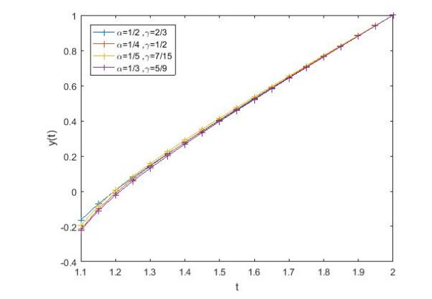
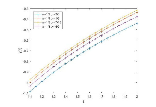
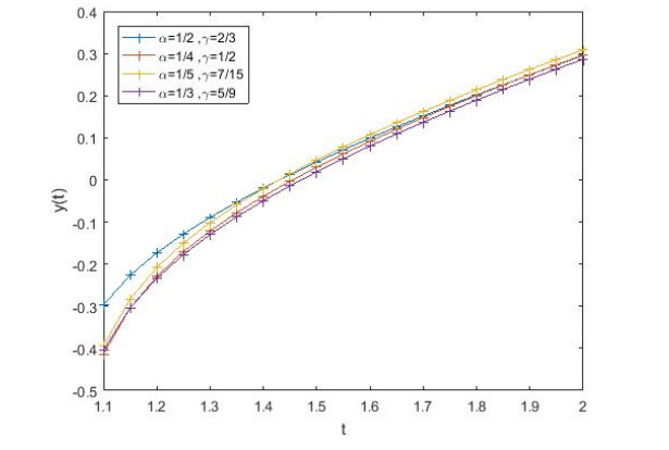
  • This article has been cited by:

    1. Chatthai Thaiprayoon, Weerawat Sudsutad, Sotiris K. Ntouyas, Mixed nonlocal boundary value problem for implicit fractional integro-differential equations via ψ-Hilfer fractional derivative, 2021, 2021, 1687-1847, 10.1186/s13662-021-03214-1
    2. Hojjat Afshari, Erdal Karapınar, A discussion on the existence of positive solutions of the boundary value problems via ψ-Hilfer fractional derivative on b-metric spaces, 2020, 2020, 1687-1847, 10.1186/s13662-020-03076-z
    3. Mohammed A. Almalahi, Mohammed S. Abdo, Satish K. Panchal, Existence and Ulam–Hyers stability results of a coupled system of ψ-Hilfer sequential fractional differential equations, 2021, 10, 25900374, 100142, 10.1016/j.rinam.2021.100142
    4. Hojjat Afshari, H. R. Marasi, Jehad Alzabut, Applications of new contraction mappings on existence and uniqueness results for implicit ϕ-Hilfer fractional pantograph differential equations, 2021, 2021, 1029-242X, 10.1186/s13660-021-02711-x
    5. Mohammed A. Almalahi, Satish K. Panchal, Some properties of implicit impulsive coupled system via φ-Hilfer fractional operator, 2021, 2021, 1687-2770, 10.1186/s13661-021-01543-4
    6. Abdelatif Boutiara, Mohammed S. Abdo, Mohammed A. Almalahi, Kamal Shah, Bahaaeldin Abdalla, Thabet Abdeljawad, Study of Sturm-Liouville boundary value problems with {p} -Laplacian by using generalized form of fractional order derivative, 2022, 7, 2473-6988, 18360, 10.3934/math.20221011
    7. Godwin Amechi Okeke, Daniel Francis, Celestin Akwumbuom Nse, A generalized contraction mapping applied in solving modified implicit \phi -Hilfer pantograph fractional differential equations, 2022, 0971-3611, 10.1007/s41478-022-00500-3
    8. Mohammed D. Kassim, Thabet Abdeljawad, Saeed M. Ali, Mohammed S. Abdo, Stability of solutions for generalized fractional differential problems by applying significant inequality estimates, 2021, 2021, 1687-1847, 10.1186/s13662-021-03533-3
    9. Dumitru Baleanu, Babak Shiri, Nonlinear higher order fractional terminal value problems, 2022, 7, 2473-6988, 7489, 10.3934/math.2022420
    10. Mohammed A. Almalahi, Satish K. Panchal, Mohammed S. Abdo, Fahd Jarad, Shrideh K. Q. Al-Omari, On Atangana–Baleanu-Type Nonlocal Boundary Fractional Differential Equations, 2022, 2022, 2314-8888, 1, 10.1155/2022/1812445
    11. K. A. Aldwoah, Mohammed A. Almalahi, Kamal Shah, Muath Awadalla, Ria H. Egami, Kinda Abuasbeh, Symmetry analysis for nonlinear fractional terminal system under w -Hilfer fractional derivative in different weighted Banach spaces, 2024, 9, 2473-6988, 11762, 10.3934/math.2024576
    12. Said Zibar, Brahim Tellab, Abdelkader Amara, Homan Emadifar, Atul Kumar, Sabir Widatalla, Existence, uniqueness and stability analysis of a nonlinear coupled system involving mixed ϕ-Riemann-Liouville and ψ-Caputo fractional derivatives, 2025, 2025, 1687-2770, 10.1186/s13661-025-01994-z
    13. Karim Chaira, Nour-Eddine El Harmouchi, Fixed point results in Menger probabilistic suprametric spaces with an application to fractional differential equations, 2025, 2025, 2730-5422, 10.1186/s13663-025-00782-9
  • Reader Comments
  • © 2020 the Author(s), licensee AIMS Press. This is an open access article distributed under the terms of the Creative Commons Attribution License (http://creativecommons.org/licenses/by/4.0)
通讯作者: 陈斌, bchen63@163.com
  • 1. 

    沈阳化工大学材料科学与工程学院 沈阳 110142

  1. 本站搜索
  2. 百度学术搜索
  3. 万方数据库搜索
  4. CNKI搜索

Metrics

Article views(4109) PDF downloads(251) Cited by(13)

Figures and Tables

Figures(3)

/

DownLoad:  Full-Size Img  PowerPoint
Return
Return

Catalog