A comparison of analytical solutions of nonlinear complex generalized Zakharov dynamical system for various definitions of the differential operator

Melih Cinar; Ismail Onder; Aydin Secer; Mustafa Bayram; Abdullahi Yusuf; Tukur Abdulkadir Sulaiman; Melih Cinar; Ismail Onder; Aydin Secer; Mustafa Bayram; Abdullahi Yusuf; Tukur Abdulkadir Sulaiman

doi:10.3934/era.2022018

Electronic Research Archive

2022, Volume 30, Issue 1: 335-361. doi: 10.3934/era.2022018

Previous Article Next Article

Research article

A comparison of analytical solutions of nonlinear complex generalized Zakharov dynamical system for various definitions of the differential operator

1.
Department of Mathematical Engineering, Yildiz Technical University, Istanbul, TURKEY
2.
Graduate School of Science and Engineering, Yildiz Technical University, Istanbul, TURKEY
3.
Department of Computer Engineering, Biruni University, Istanbul, TURKEY
4.
Department of Mathematics, Federal University Dutse, Jigawa, NIGERIA

Academic Editor: Alain Miranville

Received: 21 October 2021 Revised: 02 December 2021 Accepted: 23 December 2021 Published: 13 January 2022

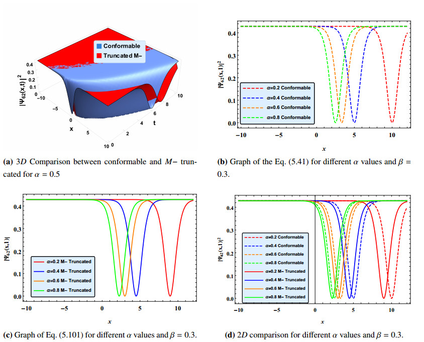
This paper considers deriving new exact solutions of a nonlinear complex generalized Zakharov dynamical system for two different definitions of derivative operators called conformable and $M-$ truncated. The system models the spread of the Langmuir waves in ionized plasma. The extended rational $sine-cosine$ and $sinh-cosh$ methods are used to solve the considered system. The paper also includes a comparison between the solutions of the models containing separately conformable and $M-$ truncated derivatives. The solutions are compared in the $2D$ and $3D$ graphics. All computations and representations of the solutions are fulfilled with the help of Mathematica 12. The methods are efficient and easily computable, so they can be applied to get exact solutions of non-linear PDEs (or PDE systems) with the different types of derivatives.

Keywords:

Zakharov dynamical system,
extended rational sine-cosine method,
extended rational sinh-cosh method exact solutions

Citation: Melih Cinar, Ismail Onder, Aydin Secer, Mustafa Bayram, Abdullahi Yusuf, Tukur Abdulkadir Sulaiman. A comparison of analytical solutions of nonlinear complex generalized Zakharov dynamical system for various definitions of the differential operator[J]. Electronic Research Archive, 2022, 30(1): 335-361. doi: 10.3934/era.2022018

Related Papers:

[1]	Najmeddine Attia, Ahmed Ghezal . Global stability and co-balancing numbers in a system of rational difference equations. Electronic Research Archive, 2024, 32(3): 2137-2159. doi: 10.3934/era.2024097
[2]	Guoqiang Dang, Qiyou Liu . Solving the conformable Huxley equation using the complex method. Electronic Research Archive, 2023, 31(3): 1303-1322. doi: 10.3934/era.2023067
[3]	Feng Ye, Xiaoting Zhang, Chunling Jiang, Bo Zeng . Comment on: "Solving the conformable Huxley equation using the complex method" [Electron. Res. Arch., 31 (2023), 1303–1322]. Electronic Research Archive, 2025, 33(1): 255-262. doi: 10.3934/era.2025013
[4]	Yantong Guo, Quansheng Wu, Xiaofeng Wang . An extension of high-order Kou's method for solving nonlinear systems and its stability analysis. Electronic Research Archive, 2025, 33(3): 1566-1588. doi: 10.3934/era.2025074
[5]	Sahar Albosaily, Wael Mohammed, Mahmoud El-Morshedy . The exact solutions of the fractional-stochastic Fokas-Lenells equation in optical fiber communication. Electronic Research Archive, 2023, 31(6): 3552-3567. doi: 10.3934/era.2023180
[6]	Jiali Shi, Zhongyi Xiang . Mathematical analysis of nonlinear combination drug delivery. Electronic Research Archive, 2025, 33(3): 1812-1835. doi: 10.3934/era.2025082
[7]	Ismail T. Huseynov, Arzu Ahmadova, Nazim I. Mahmudov . Perturbation properties of fractional strongly continuous cosine and sine family operators. Electronic Research Archive, 2022, 30(8): 2911-2940. doi: 10.3934/era.2022148
[8]	Juan Gerardo Alcázar, Carlos Hermoso, Hüsnü Anıl Çoban, Uğur Gözütok . Computation of symmetries of rational surfaces. Electronic Research Archive, 2024, 32(11): 6087-6108. doi: 10.3934/era.2024282
[9]	Mehmet Ali Özarslan, Ceren Ustaoğlu . Extended incomplete Riemann-Liouville fractional integral operators and related special functions. Electronic Research Archive, 2022, 30(5): 1723-1747. doi: 10.3934/era.2022087
[10]	Jin Li, Yongling Cheng . Barycentric rational interpolation method for solving KPP equation. Electronic Research Archive, 2023, 31(5): 3014-3029. doi: 10.3934/era.2023152

Abstract

1. Introduction

Researchers make great efforts to better model real-world problems. Fractional calculus, one of the important and fresh fields of mathematics, offers a better modeling opportunity. So, it has wide applications in various areas such as physics, biology, and chemistry, etc. There is no unique definition of the fractional derivative or integral in the literature. Some of the popular definitions of the fractional derivative are Riemann-Liouville ^[1,2], Caputo ^[3], Caputo-Fabrizio ^[4], and Atangana-Baleanu ^[5]. Besides, some scientists have introduced new definitions of differential operators such as conformable ^[6] and $M-$ truncated derivatives ^[7] in the last decade. Some works about the conformable derivative are new properties of conformable derivative ^[8], the geometric meaning of conformable derivative ^[9], price adjustment in market equilibrium ^[10], financial system analysis and hyperchaos detection ^[11], modeling neuron dynamics ^[12] and complex conformable derivative ^[13], etc. Regarding the conformable PDEs, there are many studies in the literature such as optical solution of Gerdjikov-Ivanov equation ^[14], numerical solution of Burgers' equation ^[15], wave solutions of Zakharov-Kuznetsov equation ^[16], exact solutions of space-time local fractal nonlinear evolution equations ^[17], Pochhammer-Chree equation ^[18], optical solutions of space-time nonlinear Schrodinger equation ^[19], modified KdV-Zakharov-Kuznetsov equation ^[20], Gardner equation ^[21], space-time Fokas-Lenells equation ^[22], deterministic and stochastic solutions of Schrodinger equation ^[23].

$M-$ truncated derivative, which can be thought of as generalizations of the conformable derivatives, is introduced by Sousa and Oliveira ^[7] in $2018$ . Some articles about the $M-$ truncated derivative can be listed as the longitudinal wave equation ^[24,25], $(2+1)$ dimensional Boussinesq dynamic model ^[26], Lakshmanan–Porsezian–Daniel equation ^[27], Gerdjikov-Ivanov equation ^[28], Schrodinger-Hirota equation ^[29], Sturm-Liouville problem ^[30], Hirota-Maccari system ^[31], Radhakrishnan–Kundu–Lakshmanan equation ^[31] and Biswas-Arsad model ^[32], comparative study on complex Ginzburg-Landau equation ^[33], and clinical medicine applications ^[34].

In this work, the extended rational $sine-cosine$ and $sinh-cosh$ methods ^[35,36,37] will be used to solve the non-linear complex generalized Zakharov dynamical system (NLCGZDS) ^[38]. The system is a modeling of the spread of the Langmuir waves in ionized plasma ^[39]. In order to obtain better modeling, the related system is discussed using different derivative operators called conformable and $M-$ truncated derivatives. We mainly aim to obtain novel exact solutions of the considered models to help further works in the different disciplines. Besides, we compare the obtained solutions to explain the behavior of the solutions.

The literature includes the studies on the classical NLCGZDS more. Some of them are Cauchy problem for the Zakharov system ^[40], quantum kinetics of Zakharov system ^[41], well-posedness of the system ^[42], hyperchaos investigation in the quantum Zakharov system ^[43]. The Zakharov system was solved by various methods such as time-splitting spectral method ^[44], extended trial equation method ^[45], exp-function method ^[46], local discontinuous Galerkin method ^[47], extended wave solutions of Klein-Gordon-Zakharov system ^[48] and also there is a comprehensive study on soliton solutions of Zakharov system ^[34].

The format of this article is organized as: in Section 2 some preliminaries to be used in subsequent parts are included. The mathematical analysis and the algorithm of the method are studied in Section 3. The governing model of considered PDE systems is dealt with in Section 4. In Section 5, the application of the method and the figures of the solutions of the considered equation are studied. The results and discussion can be found in Section 6. A conclusion is given in the final section.

2. Preliminaries

2.1. Conformable derivative

Definition 2.1. Let $g:[0, \infty) \rightarrow \mathbb{R}$ be a function. $\alpha$ order conformable derivative of $g(t)$ is defined as follows ^[6]:

$\begin{equation} \mathcal{D}_{t}^{\alpha}(g(t)) = \lim\limits _{h \rightarrow 0} \frac{g(t+h t^{1-\alpha})-g(t)}{h},\quad \end{equation}$

(2.1)

where $\alpha \in(0, 1], \; t > 0$ .

Theorem 2.2. ^[6]Let $g(t)$ and $h(t)$ be $\alpha$ -differentiable functions for $\alpha \in(0, 1], \; t > 0$ . Then,

1) $\mathcal{D}_{t}^{\alpha}\big(c g(t)+d h(t)\big) = c \mathcal{D}_{t}^{\alpha} g(t)+d \mathcal{D}_{t}^{\alpha} h(t), \;$ for $c, d \in \mathbb{R},$

2) $\mathcal{D}_{t}^{\alpha}\left(t^{n}\right) = n t^{n-\alpha}, \; n \in \mathbb{R}$ ,

3) If $g(t) = c$ where $c$ is a constant, then $\mathcal{D}_{t}^{\alpha}(c) = 0,$

4) $\mathcal{D}_{t}^{\alpha}\big(h(t) g(t)\big) = h(t) \mathcal{D}_{t}^{\alpha}g(t)+g(t) \mathcal{D}_{t}^{\alpha}h(t),$

5) $\mathcal{D}_{t}^{\alpha}\left(\frac{g(t)}{h(t)}\right) = \frac{h(t) \mathcal{D}_{t}^{\alpha}g(t)-g(t) \mathcal{D}_{l}^{\alpha}h(t)}{h^{2}(t)}, \quad h(t) \neq 0,$

6) If the first derivative of $g(t)$ exists, then $\mathcal{D}_{t}^{\alpha}(g(t)) = t^{1-\alpha} \frac{d g(t)}{d t}.$

2.2. $M-$ truncated derivative

Definition 2.3. The truncated Mittag-Leffler function is given as ^[7]:

$\begin{equation} { }_i \mathbb{E}_{\beta}(z) = \sum\limits_{k = 0}^{i} \frac{z^{k}}{\Gamma(\beta k+1)}, \end{equation}$

(2.2)

in which $\beta > 0$ and $z \in C$ .

Definition 2.4. Let $f:[0, \infty) \rightarrow \mathbb{R}$ be a function, the $M-$ truncated derivative of $f$ of order $\alpha \in(0, 1),$ w.r.t. $t$ is defined by ^[7]

$\begin{equation} \mathscr{D}_{M,t}^{\alpha, \beta} g(t) = \lim\limits _{\varepsilon \rightarrow 0} \frac{g\left(t+ {}_i \mathbb{E}_{\beta}\left(\varepsilon t^{-\alpha}\right)\right)-g(t)}{\varepsilon}, \end{equation}$

(2.3)

where $\beta, t > 0$ and ${}_i \mathbb{E}_{\beta}(\cdot)$ is truncated Mittag-Leffler function.

Theorem 2.5. Let $g(t)$ be $\alpha$ order differentiable function at $t_{0} > 0$ with $\alpha \in(0, 1]$ and $\beta > 0$ . Then, $g(t)$ is continuous at $t_{0}$ ^[7].

Theorem 2.6. ^[7]Let $0 < \alpha \leq 1, \beta > 0, p, q \in \mathbb{R}$ and assume that $g, h$ is $\alpha$ -differentiable at a point $t > 0.$ Then,

1) $\mathscr{D}_{M, t}^{\alpha, \beta} (p g+q h)(t) = p\; \mathscr{D}_{M, t}^{\alpha, \beta}g(t)+q\; \mathscr{D}_{M, t}^{\alpha, \beta}h(t),$ where $p, q$ are real constants,

2) $\mathscr{D}_{M, t}^{\alpha, \beta} (gh)(t) = g(t)\; \mathscr{D}_{M, t}^{\alpha, \beta}h(t)+h(t)\; \mathscr{D}_{M, t}^{\alpha, \beta}g(t),$

3) $\mathscr{D}_{M, t}^{\alpha, \beta} \left(\frac{g}{h}\right)(t) = \frac{g(t)\; \mathscr{D}_{M, t}^{\alpha, \beta}h(t)-h(t)\; \mathscr{D}_{M, t}^{\alpha, \beta}g(t)}{h(t)^{2}},$

4) $\mathscr{D}_{M, t}^{\alpha, \beta} \left(\frac{g}{h}\right)(t) = \frac{g(t)\; \mathscr{D}_{M, t}^{\alpha, \beta}h(t)-h(t)\; \mathscr{D}_{M, t}^{\alpha, \beta}g(t)}{h(t)^{2}},$

5) If $g$ is differentiable, then $\mathscr{D}_{M, t}^{\alpha, \beta}(g)(t) = \frac{t^{1-\alpha}}{\Gamma(\beta+1)} \frac{d g(t)}{d t}$ .

3. Analysis of the method

ⅰ) Let's deal with the general form of the conformable PDE system and the wave transformation as follows:

$\begin{equation} F\left( \mathcal{D}_{x}^{\alpha} \Psi,\; \mathcal{D}_{t}^{\alpha} \Psi, \; \mathcal{D}_{x}^{\alpha}\mathcal{D}_{t}^{\alpha} \Psi, \; \mathcal{D}_{t}^{\alpha} \chi, \mathcal{D}_{x}^{\alpha} \chi, \ldots\right) = 0, \end{equation}$

(3.1)

$\begin{equation} G\left( \mathcal{D}_{x}^{\alpha} \Psi,\; \mathcal{D}_{t}^{\alpha} \Psi, \; \mathcal{D}_{x}^{\alpha}\mathcal{D}_{t}^{\alpha} \Psi, \; \mathcal{D}_{t}^{\alpha} \chi, \mathcal{D}_{x}^{\alpha} \chi, \ldots\right) = 0, \end{equation}$

(3.2)

and

$\begin{equation} \Psi(x, t) = Y(\xi) e^{i \phi},\; \xi = \frac{c_1 x^\alpha+c_2 t^\alpha}{\alpha}, \; \phi = \frac{c_3 x^{\alpha }+c_4 t^{\alpha }}{\alpha }, \; \chi(x,t) = Q(\xi). \end{equation}$

(3.3)

ⅱ) Consider the general form of the local $M-$ truncated PDE system and the wave transformation as follows:

$\begin{equation} F\left( \mathscr{D}_{M, x}^{\alpha, \beta} \Psi,\; \mathscr{D}_{M, t}^{\alpha, \beta} \Psi, \; \mathscr{D}_{M, x}^{\alpha, \beta}\mathscr{D}_{M, t}^{\alpha, \beta} \Psi, \; \mathscr{D}_{M, x}^{\alpha, \beta} \chi, \mathscr{D}_{M, t}^{\alpha, \beta} \chi, \ldots\right) = 0, \end{equation}$

(3.4)

$\begin{equation} G\left( \mathscr{D}_{M, x}^{\alpha, \beta} \Psi,\; \mathscr{D}_{M, t}^{\alpha, \beta} \Psi, \; \mathscr{D}_{M, x}^{\alpha, \beta}\mathscr{D}_{M, t}^{\alpha, \beta} \Psi, \; \mathscr{D}_{M, x}^{\alpha, \beta} \chi, \mathscr{D}_{M, t}^{\alpha, \beta} \chi, \ldots\right) = 0, \end{equation}$

(3.5)

and

$\begin{equation} \begin{aligned} \Psi(x, t) = Y(\xi) e^{i \phi},\; &\chi(x,t) = Q(\xi)\;,\\ \xi = \frac{\Gamma (\beta +1)\big(c_1 x^\alpha+c_2 t^\alpha \big)}{\alpha} , \; &\phi = \frac{ \Gamma (\beta +1)\big(c_3 x^{\alpha }+c_4 t^\alpha\big)}{\alpha }, \end{aligned} \end{equation}$

(3.6)

where $\Psi(x, t)$ and $\chi(x, t)$ are the unknown functions, $\mathcal{D}_{*}^{\alpha}$ and $\mathscr{D}_{M, *}^{\alpha, \beta}$ are the $\alpha$ order conformable and $M-$ truncated derivative operators with respect to $*\; (x$ or $t),$ respectively.

Substituting the wave transformations to the PDE systems yields the following nonlinear ordinary differential equation systems:

$\begin{equation} K\left(Y, Y^{\prime}, Y^{\prime \prime}, \ldots,Q, Q^{\prime},Q^{\prime \prime}, \ldots\right) = 0, \end{equation}$

(3.7)

$\begin{equation} L\left(Y, Y^{\prime}, Y^{\prime \prime}, \ldots,Q ,Q^{\prime},Q^{\prime \prime}, \ldots\right) = 0, \end{equation}$

(3.8)

where $Y$ and $Q$ are the unknown functions of $\xi$ and the superscript indicates the derivative of the functions with respect to $\xi$ .

3.1. Extended rational $sine-cosine$ method

Step 1: Assume that the ODE system in (3.7) and (3.8) have the solutions as follows:

$\begin{equation} u(\psi) = \frac{\omega_{0} \sin (\mu \psi)}{\omega_{2}+\omega_{1} \cos (\mu \psi)}, \; \cos (\mu \psi) \neq-\frac{\omega_{2}}{\omega_{1}}, \end{equation}$

(3.9)

$\begin{equation} u(\psi) = \frac{\omega_{0} \cos (\mu \psi)}{\omega_{2}+\omega_{1} \sin (\mu \psi)}, \; \sin (\mu \psi) \neq-\frac{\omega_{2}}{\omega_{1}}. \end{equation}$

(3.10)

where $\omega_0, \omega_1$ , and $\omega_2$ are parameters to be found in the next step. $\mu$ is the wave number to be also determined after substitution.

Step 2: Substitute the (3.9) or the (3.10) to the (3.7) and the (3.8). After collecting all terms with the same powers of $\cosh (\mu \psi)$ or $\sinh (\mu \psi)$ , we derive a set of algebraic equations by equating all the coefficients of $\cosh (\mu \psi)$ or $\sinh (\mu \psi)$ to zero. In order to find the unknowns ( $\omega_0, \omega_1, \omega_2$ and $\mu$ ), the system can be solved by Maple, Mathematica, etc.

Step 3: Substitute the values of $\omega_0, \omega_1, \omega_2, \psi$ and $\mu$ into (3.9) or (3.10), the solutions of the ODE system in (3.7) and (3.8) can be found.

3.2. Extended rational $sinh-cosh$ method

Step 1: Suppose that the ODE system in (3.7) and (3.8) have the solutions as follows:

$\begin{equation} u(\psi) = \frac{\omega_{0} \sinh (\mu \psi)}{\omega_{2}+\omega_{1} \cosh (\mu \psi)}, \; \cosh (\mu \psi) \neq-\frac{\omega_{2}}{\omega_{1}}, \end{equation}$

(3.11)

$\begin{equation} u(\psi) = \frac{\omega_{0} \cosh (\mu \psi)}{\omega_{2}+\omega_{1} \sinh (\mu \psi)}, \; \sinh (\mu \psi) \neq-\frac{\omega_{2}}{\omega_{1}}, \end{equation}$

(3.12)

where $\omega_0, \omega_1$ , and $\omega_2$ are parameters to be found in the next step. $\mu$ is the wave number to be also determined after substitution.

Step 2: Substitute the (3.11) or the (3.12) to the (3.7) and the (3.8). After collecting all terms with the same powers of $\cosh (\mu \psi)$ or $\sinh (\mu \psi)$ , we derive a set of algebraic equations by equating all the coefficients of $\cosh (\mu \psi)$ or $\sinh (\mu \psi)$ to zero. In order to find the unknowns ( $\omega_0, \omega_1, \omega_2$ and $\mu$ ), the system can be solved by Maple, Mathematica, etc.

Step 3: Substitute the values of $\omega_0, \omega_1, \omega_2, \psi$ and $\mu$ into (3.11) or (3.12), the solutions of the ODE system in (3.7) and (3.8) can be found.

4. Governing models

In this section, we consider the NLCGZDS with respect to different definitions of derivatives ^[49]:

4.1. Model with conformable derivative

In conformable derivative, the considered equation might be written as ^[49]:

$\begin{equation} \left\{\begin{array}{l} i\; \mathcal{D}_{t}^{\alpha}\Psi+\Psi_{x x}-2 \delta|\Psi|^{2} \Psi+2 \chi \Psi = 0, \\ \mathcal{D}_{t}^{2\alpha}\chi-\chi_{x x}+\left(|\Psi|^{2}\right)_{x x} = 0. \end{array}\right. \end{equation}$

(4.1)

For conformable derivative, the following wave transformations are employed:

$\begin{equation} \Psi(x, t) = Y(\xi) e^{i \phi}, \; \chi(x,t) = Q(\xi),\; \xi = x- \frac{2kt^\alpha}{\alpha} , \; \phi = \frac{c t^{\alpha }}{\alpha }+k x. \end{equation}$

(4.2)

4.2. Model with $M-$ truncated derivative

In $M-$ truncated derivative, the considered equation might be written as ^[49]:

$\begin{equation} \left\{\begin{array}{l} i\; { }_{i} \mathscr{D}_{M,t}^{\alpha, \beta}\Psi+\Psi_{x x}-2 \delta|\Psi|^{2} \Psi+2 \chi \Psi = 0, \\ { }_{i} \mathscr{D}_{M,t}^{2\alpha, \beta}\chi-\chi_{x x}+\left(|\Psi|^{2}\right)_{x x} = 0. \end{array}\right. \end{equation}$

(4.3)

For $M-$ truncated derivative, the following wave transformations are employed:

$\begin{equation} \Psi(x, t) = Y(\xi) e^{i \phi},\; \chi(x,t) = Q(\xi),\; \xi = x-\frac{2 k \Gamma (\beta +1) t^{\alpha }}{\alpha },\; \phi = \frac{c \Gamma (\beta +1) t^{\alpha }}{\alpha }+k x. \end{equation}$

(4.4)

4.3. Solutions of the governing models

Applying the wave transformations in (4.2) and (4.4) to the (4.1) and (4.3), respectively, we obtain the following ODE system:

$\begin{equation} \left\{\begin{array}{l} Y^{\prime \prime}-\left(c+k^{2}\right) Y-2 \delta Y^{3}+2 Y Q = 0, \\ \left(4 k^{2}-1\right) Q^{\prime \prime}+\left(Y^{2}\right)^{\prime \prime} = 0. \end{array}\right. \end{equation}$

(4.5)

Integrating two times the second equation in the (4.5) and supposing the integration constant is zero, we get:

$\begin{equation} Q(\xi) = \frac{Y^2}{1-4k^2}. \end{equation}$

(4.6)

Substituting $Q(\xi)$ to the first equation in the (4.5), we get:

$\begin{equation} Y^{\prime \prime}-\left(c+k^{2}\right) Y+\left(\frac{2}{1-4 k^{2}}-2 \delta\right) Y^{3} = 0. \end{equation}$

(4.7)

Balancing the highest order derivative term and the nonlinear term, we derive $N + 2 = 3N \Rightarrow N = 1.$

5. Application

5.1. Conformable Zakharov system

5.1.1. Application of the extended rational $sine-cosine$ method to the conformable Zakharov system

Assume that the (4.7) has the solution in the form:

$\begin{equation} Y \left( \xi \right) = {\frac {\omega_{{0}}\sin \left[ \mu\,\xi \right]}{\omega_{{2}}+\omega_{{1}}\cos \left[ \mu\,\xi \right] }}. \end{equation}$

(5.1)

Substituting (5.1) into the (4.7) ODE to get the algebraic equations formed by collecting all terms comprising the same powers of $cos[\mu\, \xi]^m$ .

$\begin{equation} \begin{split} cos(\mu\,\xi)^2 :\quad &-4 c k^2 \omega _0 \omega _1^2+c \omega _0 \omega _1^2-2 \delta \omega _0^3-4 k^4 \omega _0 \omega _1^2+8 \delta k^2 \omega _0^3+k^2 \omega _0 \omega _1^2+2 \omega _0^3 = 0,\\ cos(\mu\,\xi)^1 :\quad &-16 c k^2 \omega _0 \omega _1 \omega _2+4 c \omega _0 \omega _1 \omega _2-16 k^4 \omega _0 \omega _1 \omega _2+8 k^2 \mu ^2 \omega _0 \omega _1 \omega _2+4 k^2 \omega _0 \omega _1 \omega _2 \\ &-2 \mu ^2 \omega _0 \omega _1 \omega _2 = 0,\\ cos(\mu\,\xi)^0 :\quad &-4 c k^2 \omega _0 \omega _1^2-16 c k^2 \omega _0 \omega _2^2+c \omega _0 \omega _1^2+4 c \omega _0 \omega _2^2+6 \delta \omega _0^3-4 k^4 \omega _0 \omega _1^2\\ &-16 k^4 \omega _0 \omega _2^2 -24 \delta k^2 \omega _0^3+32 k^2 \mu ^2 \omega _0 \omega _1^2-16 k^2 \mu ^2 \omega _0 \omega _2^2+k^2 \omega _0 \omega _1^2+4 k^2 \omega _0 \omega _2^2\\ &-8 \mu ^2 \omega _0 \omega _1^2+4 \mu ^2 \omega _0 \omega _2^2-6 \omega _0^3 = 0. \end{split} \end{equation}$

(5.2)

After solving the system of equations in the (5.2) via Mathematica, the following cases are derived:

Case 1:

$\begin{equation} \mu = \pm {\frac{\sqrt{c+k^2}}{\sqrt{2}}},\;\omega_{{0}} = \pm{\frac{i \sqrt{4 k^2-1} \sqrt{c+k^2}}{\sqrt{\delta \left(2-8 k^2\right)-2}}\omega _1},\;\omega_{{1}} = \omega_{{1} },\;\omega_{{2}} = 0 . \end{equation}$

(5.3)

Substituting the parameters in Case 1 to the (5.1), the solutions of (4.7) can be derived:

$\begin{equation} Y_{1}(\xi) = \pm { \frac{i \sqrt{4 k^2-1} \sqrt{c+k^2}}{\sqrt{\delta \left(2-8 k^2\right)-2}} \tan \left[\frac{\xi \sqrt{c+k^2}}{\sqrt{2}}\right] }. \end{equation}$

(5.4)

Considering the (5.4) and the (4.2), the following solutions of the conformable Zakharov system are obtained:

$\begin{equation} \Psi_{11}(x,t) = \frac{i \sqrt{4 k^2-1} \sqrt{c+k^2}}{\sqrt{\delta \left(2-8 k^2\right)-2}} \tan \left[\frac{\left(x-\frac{2 k t^{\alpha }}{\alpha }\right) \sqrt{c+k^2}}{\sqrt{2}}\right] e^{i \left(\frac{c t^{\alpha }}{\alpha }+k x\right)}, \end{equation}$

(5.5)

$\begin{equation} \Psi_{12}(x,t) = -\frac{i \sqrt{4 k^2-1} \sqrt{c+k^2}}{\sqrt{\delta \left(2-8 k^2\right)-2}} \tan \left[\frac{\left(x-\frac{2 k t^{\alpha }}{\alpha }\right) \sqrt{c+k^2}}{\sqrt{2}}\right] e^{i \left(\frac{c t^{\alpha }}{\alpha }+k x\right)} , \end{equation}$

(5.6)

$\begin{equation} \chi_{11}(x,t) = \chi_{12}(x,t) = -\frac{\left(4 k^2-1\right) \left(c+k^2\right) }{\left(1-4 k^2\right) \left(\delta \left(2-8 k^2\right)-2\right)} \tan ^2\left[\frac{\sqrt{c+k^2} \left(x-\frac{2 k t^{\alpha }}{\alpha }\right)}{\sqrt{2}}\right]. \end{equation}$

(5.7)

These solutions are corresponding to trigonometric soliton solutions in the literature and valid for $\left(c + k^{2}\right) > 0$ .

Case 2:

$\begin{equation} \mu = \pm{\sqrt{2} \sqrt{c+k^2} },\omega_{{0}} = \pm{\frac{i \sqrt{4 k^2-1} \sqrt{c+k^2}}{\sqrt{\delta \left(2-8 k^2\right)-2}}\omega _1},\omega_{{2}} = \omega_{{2}},\omega_{{1}} = \pm \omega_{{2}}. \end{equation}$

(5.8)

Substituting the parameters in Case 2 to the (5.1), the solutions of (4.7) can be derived:

$\begin{equation} Y_{2}(\xi) = \pm{\frac{i \sqrt{4 k^2-1} \sqrt{c+k^2}}{\sqrt{\delta \left(2-8 k^2\right)-2} } \frac{ \sin \left[\sqrt{2} \xi \sqrt{c+k^2}\right]}{\left[\omega_{2} \cos \left(\sqrt{2} \xi \sqrt{c+k^2}\right)+\omega_{1}\right]} }. \end{equation}$

(5.9)

Considering the (5.9) and the (4.2), the following solutions of the conformable Zakharov system are obtained:

$\begin{equation} \Psi_{21}(x,t) = \frac{i \sqrt{4 k^2-1} \sqrt{c+k^2}}{\sqrt{\delta \left(2-8 k^2\right)-2} } {\frac{ \sin \left[\sqrt{2} \sqrt{c+k^2} \left(x-\frac{2 k t^{\alpha }}{\alpha }\right)\right] e^{i \left(\frac{c t^{\alpha }}{\alpha }+k x\right)}}{\left[1+ \cos \left(\sqrt{2} \sqrt{c+k^2} \left(x-\frac{2 k t^{\alpha }}{\alpha }\right)\right)\right]} }, \end{equation}$

(5.10)

$\begin{equation} \Psi_{22}(x,t) = -\frac{i \sqrt{4 k^2-1} \sqrt{c+k^2}}{\sqrt{\delta \left(2-8 k^2\right)-2} } {\frac{ \sin \left[\sqrt{2} \sqrt{c+k^2} \left(x-\frac{2 k t^{\alpha }}{\alpha }\right)\right] e^{i \left(\frac{c t^{\alpha }}{\alpha }+k x\right)}}{\left[1+ \cos \left(\sqrt{2} \sqrt{c+k^2} \left(x-\frac{2 k t^{\alpha }}{\alpha }\right)\right)\right]} }, \end{equation}$

(5.11)

$\begin{equation} \Psi_{23}(x,t) = -\frac{i \sqrt{4 k^2-1} \sqrt{c+k^2}}{\sqrt{\delta \left(2-8 k^2\right)-2} } {\frac{ \sin \left[\sqrt{2} \sqrt{c+k^2} \left(x-\frac{2 k t^{\alpha }}{\alpha }\right)\right] e^{i \left(\frac{c t^{\alpha }}{\alpha }+k x\right)}}{\left[1- \cos \left(\sqrt{2} \sqrt{c+k^2} \left(x-\frac{2 k t^{\alpha }}{\alpha }\right)\right)\right]} }, \end{equation}$

(5.12)

$\begin{equation} \Psi_{24}(x,t) = \frac{i \sqrt{4 k^2-1} \sqrt{c+k^2}}{\sqrt{\delta \left(2-8 k^2\right)-2} } {\frac{ \sin \left[\sqrt{2} \sqrt{c+k^2} \left(x-\frac{2 k t^{\alpha }}{\alpha }\right)\right] e^{i \left(\frac{c t^{\alpha }}{\alpha }+k x\right)}}{\left[1- \cos \left(\sqrt{2} \sqrt{c+k^2} \left(x-\frac{2 k t^{\alpha }}{\alpha }\right)\right)\right]} }, \end{equation}$

(5.13)

$\begin{equation} \chi_{21}(x,t) = \chi_{22}(x,t) = -\frac{\left(4 k^2-1\right) \left(c+k^2\right) }{\left(1-4 k^2\right) \left(\delta \left(2-8 k^2\right)-2\right) }\frac{\sin ^2\left[\sqrt{2} \sqrt{c+k^2} \left(x-\frac{2 k t^{\alpha }}{\alpha }\right)\right]}{\left[1+\cos \left(\sqrt{2} \sqrt{c+k^2} \left(x-\frac{2 k t^{\alpha }}{\alpha }\right)\right)\right]^2}, \end{equation}$

(5.14)

$\begin{equation} \chi_{23}(x,t) = \chi_{24}(x,t) = -\frac{\left(4 k^2-1\right) \left(c+k^2\right) }{\left(1-4 k^2\right) \left(\delta \left(2-8 k^2\right)-2\right) }\frac{\sin ^2\left[\sqrt{2} \sqrt{c+k^2} \left(x-\frac{2 k t^{\alpha }}{\alpha }\right)\right]}{\left[1-\cos \left(\sqrt{2} \sqrt{c+k^2} \left(x-\frac{2 k t^{\alpha }}{\alpha }\right)\right)\right]^2}. \end{equation}$

(5.15)

These solutions are valid for $(c + k^{2}) > 0$ .

Suppose that solutions of the (4.7) is in the form:

$\begin{equation} Y \left( \xi \right) = {\frac {\omega_{{0}}\cos \left[ \mu\,\xi \right]}{\omega_{{2}}+\omega_{{1}}\sin \left[ \mu\,\xi \right] }}. \end{equation}$

(5.16)

Substituting the (5.16) into the (4.7) to get the algebraic equations formed by collecting all terms comprising the same powers of $sin[\mu\, \xi]^m$ .

$\begin{equation} \begin{split} sin(\mu\,\xi)^2 :\quad& 2 \omega_0 \omega_1^2 c k^2-\frac{1}{2} \omega_0 \omega_1^2 c+\omega_0^3 \delta +2 \omega_0 \omega_1^2 k^4-4 \omega_0^3 \delta k^2-\frac{1}{2} \omega_0 \omega_1^2 k^2-\omega_0^3 = 0, \\ sin(\mu\,\xi)^1 :\quad & -8 \omega_0 \omega_1 \omega_2 c k^2+2 \omega_0 \omega_1 \omega_2 c-8 \omega_0 \omega_1 \omega_2 k^4+4 \omega_0 \omega_1 \omega_2 k^2 \mu ^2+2 \omega_0 \omega_1 \omega_2 k^2\\ &-\omega_0 \omega_1 \omega_2 \mu ^2 = 0,\\ sin(\mu\,\xi)^0 :\quad &-2 \omega_0 \omega_1^2 c k^2-8 \omega_0 \omega_2^2 c k^2+\frac{1}{2} \omega_0 \omega_1^2 c+2 \omega_0 \omega_2^2 c+3 \omega_0^3 \delta -2 \omega_0 \omega_1^2 k^4\\ &-8 \omega_0 \omega_2^2 k^4-12 \omega_0^3 \delta k^2+16 \omega_0 \omega_1^2 k^2 \mu ^2-8 \omega_0 \omega_2^2 k^2 \mu ^2+\frac{1}{2} \omega_0 \omega_1^2 k^2\\ &+2 \omega_0 \omega_2^2 k^2-4 \omega_0 \omega_1^2 \mu ^2+2 \omega_0 \omega_2^2 \mu ^2-3 \omega_0^3 = 0. \end{split} \end{equation}$

(5.17)

After solving the system of equations in the (5.17) via Mathematica, the following cases are derived:

Case 3:

$\begin{equation} \mu = \pm \frac{\sqrt{c+k^2}}{\sqrt{2}},\omega_{{0}} = \pm\frac{i \omega_1 \sqrt{4 k^2-1} \sqrt{c+k^2}}{\sqrt{\delta \left(2-8 k^2\right)-2}} ,\omega_{{1}} = \omega_{{1} },\omega_{{2}} = 0. \end{equation}$

(5.18)

Substituting the parameters in Case 3 to the (5.1), the solutions of (4.7) can be derived:

$\begin{equation} Y_{3}(\xi) = \pm \frac{i \sqrt{4 k^2-1} \sqrt{c+k^2} }{\sqrt{\delta \left(2-8 k^2\right)-2}}\cot \left[\frac{\xi \sqrt{c+k^2}}{\sqrt{2}}\right]. \end{equation}$

(5.19)

Considering the (5.19) and the (4.2), the following solutions of the conformable Zakharov system are obtained:

$\begin{equation} \Psi_{31}(x,t) = \frac{i \sqrt{4 k^2-1} \sqrt{c+k^2} }{\sqrt{\delta \left(2-8 k^2\right)-2}}\cot \left[\frac{ (x-\frac{2 k t^{\alpha }}{\alpha }) \sqrt{c+k^2}}{\sqrt{2}}\right]e^{i \left(\frac{c t^{\alpha }}{\alpha }+k x\right)}, \end{equation}$

(5.20)

$\begin{equation} \Psi_{32}(x,t) = -\frac{i \sqrt{4 k^2-1} \sqrt{c+k^2} }{\sqrt{\delta \left(2-8 k^2\right)-2}}\cot \left[\frac{ (x-\frac{2 k t^{\alpha }}{\alpha }) \sqrt{c+k^2}}{\sqrt{2}}\right]e^{i \left(\frac{c t^{\alpha }}{\alpha }+k x\right)}, \end{equation}$

(5.21)

$\begin{equation} \chi_{31}(x,t) = \chi_{32}(x,t) = \frac{\left(4 k^2-1\right) \left(c+k^2\right) }{\left(1-4 k^2\right) \left(\delta \left(2-8 k^2\right)-2\right)}\cot ^2\left[\frac{\sqrt{c+k^2} \left(x-\frac{2 k t^{\alpha }}{\alpha }\right)}{\sqrt{2}}\right]. \end{equation}$

(5.22)

These solutions are corresponding to trigonometric soliton solutions in the literature and valid for $(c + k^{2}) > 0$ .

Case 4:

$\begin{equation} \mu = \pm \sqrt{2} \sqrt{c+k^2},\omega_{{0}} = \pm\frac{i \omega_1 \sqrt{4 k^2-1} \sqrt{c+k^2}}{\sqrt{\delta \left(2-8 k^2\right)-2}} ,\omega_{{2}} = \omega_{{2}},\omega_{{1}} = \pm \omega_{{2}}. \end{equation}$

(5.23)

Substituting the parameters in Case 4 to the (5.1), the solutions of (4.7) can be derived:

$\begin{equation} Y_{4}(\xi) = \pm\frac{i \sqrt{4 k^2-1} \sqrt{c+k^2} }{\sqrt{\delta \left(2-8 k^2\right)-2}} {\frac{\cos\left[\sqrt{2} \xi \sqrt{c+k^2} \right]}{\omega_{{2}}\pm\omega_{{1}}\sin \left[\sqrt{2} \xi \sqrt{c+k^2} \right]} }. \end{equation}$

(5.24)

Considering the (5.24) and the (4.2), the following solutions of the conformable Zakharov system are obtained:

$\begin{equation} \Psi_{41}(x,t) = \frac{i \sqrt{4 k^2-1} \sqrt{c+k^2} }{\sqrt{\delta \left(2-8 k^2\right)-2}} {\frac{\cos\left[\left(x-\frac{2 k t^{\alpha }}{\alpha }\right) \sqrt{2} \sqrt{c+k^2} \right] e^{i \left(\frac{c t^{\alpha }}{\alpha }+k x\right)}}{1+\sin \left[ \left(x-\frac{2 k t^{\alpha }}{\alpha }\right) \sqrt{2} \sqrt{c+k^2} \right]} }, \end{equation}$

(5.25)

$\begin{equation} \Psi_{42}(x,t) = -\frac{i \sqrt{4 k^2-1} \sqrt{c+k^2} }{\sqrt{\delta \left(2-8 k^2\right)-2}} {\frac{\cos\left[\left(x-\frac{2 k t^{\alpha }}{\alpha }\right) \sqrt{2} \sqrt{c+k^2} \right] e^{i \left(\frac{c t^{\alpha }}{\alpha }+k x\right)}}{1+\sin \left[ \left(x-\frac{2 k t^{\alpha }}{\alpha }\right) \sqrt{2} \sqrt{c+k^2} \right]} }, \end{equation}$

(5.26)

$\begin{equation} \Psi_{43}(x,t) = -\frac{i \sqrt{4 k^2-1} \sqrt{c+k^2} }{\sqrt{\delta \left(2-8 k^2\right)-2}} {\frac{\cos\left[\left(x-\frac{2 k t^{\alpha }}{\alpha }\right) \sqrt{2} \sqrt{c+k^2} \right] e^{i \left(\frac{c t^{\alpha }}{\alpha }+k x\right)}}{1-\sin \left[ \left(x-\frac{2 k t^{\alpha }}{\alpha }\right) \sqrt{2} \sqrt{c+k^2} \right]} }, \end{equation}$

(5.27)

$\begin{equation} \Psi_{44}(x,t) = \frac{i \sqrt{4 k^2-1} \sqrt{c+k^2} }{\sqrt{\delta \left(2-8 k^2\right)-2}} {\frac{\cos\left[\left(x-\frac{2 k t^{\alpha }}{\alpha }\right) \sqrt{2} \sqrt{c+k^2} \right] e^{i \left(\frac{c t^{\alpha }}{\alpha }+k x\right)}}{1-\sin \left[ \left(x-\frac{2 k t^{\alpha }}{\alpha }\right) \sqrt{2} \sqrt{c+k^2} \right]} }, \end{equation}$

(5.28)

$\begin{equation} \chi_{41}(x,t) = \chi_{42}(x,t) = -\frac{\left(4 k^2-1\right) \left(c+k^2\right) }{\left(1-4 k^2\right) \left(\delta \left(2-8 k^2\right)-2\right) }\frac{\cos ^2\left[\sqrt{2} \sqrt{c+k^2} \left(x-\frac{2 k t^{\alpha }}{\alpha }\right)\right]}{\left[1+\sin \left(\sqrt{2} \sqrt{c+k^2} \left(x-\frac{2 k t^{\alpha }}{\alpha }\right)\right)\right]^2}, \end{equation}$

(5.29)

$\begin{equation} \chi_{43}(x,t) = \chi_{44}(x,t) = -\frac{\left(4 k^2-1\right) \left(c+k^2\right) }{\left(1-4 k^2\right) \left(\delta \left(2-8 k^2\right)-2\right) }\frac{\cos ^2\left[\sqrt{2} \sqrt{c+k^2} \left(x-\frac{2 k t^{\alpha }}{\alpha }\right)\right]}{\left[1-\sin \left(\sqrt{2} \sqrt{c+k^2} \left(x-\frac{2 k t^{\alpha }}{\alpha }\right)\right)\right]^2}. \end{equation}$

(5.30)

These solutions are valid for $(c+ k^{2}) > 0$ .

5.1.2. Application of the extended rational $sinh-cosh$ method to the conformable Zakharov system

Suppose that solutions of the (4.7) is in the form:

$\begin{equation} Y \left( \xi \right) = {\frac {\omega_{{0}}\sinh \left[ \mu\,\xi \right]}{\omega_{{2}}+\omega_{{1}}\cosh \left[ \mu\,\xi \right] }}. \end{equation}$

(5.31)

Substituting the (5.31) into the (4.7) to get the algebraic equations formed by collecting all terms comprising the same powers of $cosh[\mu\, \xi]^m$ .

$\begin{equation} \begin{split} cosh(\mu\,\xi)^2 :\quad& -4 \omega_0 \omega_1^2 c k^2+\omega_0 \omega_1^2 c+2 \omega_0^3 \delta -4 \omega_0 \omega_1^2 k^4-8 \omega_0^3 \delta k^2+\omega_0 \omega_1^2 k^2-2 \omega_0^3, \\ cosh(\mu\,\xi)^1 :\quad & -16 \omega_0 \omega_1 \omega_2 c k^2+4 \omega_0 \omega_1 \omega_2 c-16 \omega_0 \omega_1 \omega_2 k^4-8 \omega_0 \omega_1 \omega_2 k^2 \mu ^2+4 \omega_0 \omega_1 \omega_2 k^2\\ &+2 \omega_0 \omega_1 \omega_2 \mu ^2 = 0,\\ cosh(\mu\,\xi)^0 :\quad & -4 \omega_0 \omega_1^2 c k^2-16 \omega_0 \omega_2^2 c k^2+\omega_0 \omega_1^2 c+4 \omega_0 \omega_2^2 c-6 \omega_0^3 \delta -4 \omega_0 \omega_1^2 k^4-16 \omega_0 \omega_2^2 k^4\\ &+24 \omega_0^3 \delta k^2-32 \omega_0 \omega_1^2 k^2 \mu ^2+16 \omega_0 \omega_2^2 k^2 \mu ^2+\omega_0 \omega_1^2 k^2+4 \omega_0 \omega_2^2 k^2+8 \omega_0 \omega_1^2 \mu ^2\\ &-4 \omega_0 \omega_2^2 \mu ^2+6 \omega_0^3 = 0. \end{split} \end{equation}$

(5.32)

After solving the system of equations in the (5.32) via Mathematica, the following cases are derived:

Case 5:

$\begin{equation} \mu = \pm{\frac{\sqrt{-c-k^2}}{\sqrt{2}}},\omega_{{0}} = \pm{\frac{i \omega_1 \sqrt{4 k^2-1} \sqrt{c+k^2}}{\sqrt{\delta \left(8 k^2-2\right)+2}}},\omega_{{1}} = \omega_{{1}},\omega_{ {2}} = 0. \end{equation}$

(5.33)

Substituting the parameters in Case 5 to the (5.1), the solutions of (4.7) can be derived:

$\begin{equation} Y_{5}(\xi) = \pm \frac{i \sqrt{4 k^2-1} \sqrt{c+k^2}}{\sqrt{\delta \left(8 k^2-2\right)+2}} \tanh \left[\frac{\xi \sqrt{-c-k^2}}{\sqrt{2}} \right] . \end{equation}$

(5.34)

Considering the (5.34) and the (4.2), the following solutions of the conformable Zakharov system are obtained:

$\begin{equation} \Psi_{51}(x,t) = \frac{i \sqrt{4 k^2-1} \sqrt{c+k^2}}{\sqrt{\delta \left(8 k^2-2\right)+2}} \tanh \left[\frac{(x-\frac{2 k t^{\alpha }}{\alpha }) \sqrt{-c-k^2}}{\sqrt{2}} \right]e^{i \left(\frac{c t^{\alpha }}{\alpha }+k x\right)}, \end{equation}$

(5.35)

$\begin{equation} \Psi_{52}(x,t) = -\frac{i \sqrt{4 k^2-1} \sqrt{c+k^2}}{\sqrt{\delta \left(8 k^2-2\right)+2}} \tanh \left[\frac{(x-\frac{2 k t^{\alpha }}{\alpha } ) \sqrt{-c-k^2}}{\sqrt{2}} \right]e^{i \left(\frac{c t^{\alpha }}{\alpha }+k x\right)}, \end{equation}$

(5.36)

$\begin{equation} \chi_{51}(x,t) = \chi_{52}(x,t) = -\frac{\left(4 k^2-1\right) \left(c+k^2\right) }{\left(1-4 k^2\right) \left(\delta \left(8 k^2-2\right)+2\right)}\tanh ^2\left[\frac{\sqrt{-c-k^2} \left(x-\frac{2 k t^{\alpha }}{\alpha }\right)}{\sqrt{2}}\right]. \end{equation}$

(5.37)

These solutions are corresponding to dark soliton solutions in the literature and valid for $(-c- k^{2}) > 0$ and $\left(4 k^2-1\right) \left(c+k^2\right) \left(\delta \left(8 k^2-2\right)+2\right) < 0$ .

Case 6:

$\begin{equation} \mu = \pm{\sqrt{2} \sqrt{-c-k^2}},\omega_{{0}} = \pm{\frac{i \omega_1 \sqrt{4 k^2-1} \sqrt{c+k^2}}{\sqrt{\delta \left(8 k^2-2\right)+2}}},\omega_{{2}} = \omega_{{2}},\omega_{{1}} = \pm \omega_{{2}} . \end{equation}$

(5.38)

Substituting the parameters in Case 6 to the (5.1), the solutions of (4.7) can be derived:

$\begin{equation} Y_{6}(\xi) = \pm \frac{i \sqrt{4 k^2-1} \sqrt{c+k^2} }{\sqrt{\delta \left(8 k^2-2\right)+2} } {\frac{\sinh \left[\sqrt{2} \xi \sqrt{-c-k^2} \right]}{\omega_{{2}}\pm\omega_{{1}}\cosh \left[\sqrt{2} \xi \sqrt{-c-k^2} \right]} }. \end{equation}$

(5.39)

Considering the (5.39) and the (4.2), the following solutions of the conformable Zakharov system are obtained:

$\begin{equation} \Psi_{61}(x,t) = \frac{i \sqrt{4 k^2-1} \sqrt{c+k^2} }{\sqrt{\delta \left(8 k^2-2\right)+2} } {\frac{\sinh \left[ (x-\frac{2 k t^{\alpha }}{\alpha }) \sqrt{2} \sqrt{-c-k^2} \right] e^{i \left(\frac{c t^{\alpha }}{\alpha }+k x\right)}}{1+\cosh \left[ (x-\frac{2 k t^{\alpha }}{\alpha })\sqrt{2} \sqrt{-c-k^2} \right]} }, \end{equation}$

(5.40)

$\begin{equation} \Psi_{62}(x,t) = -\frac{i \sqrt{4 k^2-1} \sqrt{c+k^2} }{\sqrt{\delta \left(8 k^2-2\right)+2} } {\frac{\sinh \left[ (x-\frac{2 k t^{\alpha }}{\alpha })\sqrt{2} \sqrt{-c-k^2} \right] e^{i \left(\frac{c t^{\alpha }}{\alpha }+k x\right)}}{1+\cosh \left[ (x-\frac{2 k t^{\alpha }}{\alpha }) \sqrt{2} \sqrt{-c-k^2} \right]} }, \end{equation}$

(5.41)

$\begin{equation} \Psi_{63}(x,t) = -\frac{i \sqrt{4 k^2-1} \sqrt{c+k^2} }{\sqrt{\delta \left(8 k^2-2\right)+2} } {\frac{\sinh \left[ (x-\frac{2 k t^{\alpha }}{\alpha })\sqrt{2} \sqrt{-c-k^2} \right] e^{i \left(\frac{c t^{\alpha }}{\alpha }+k x\right)}}{1-\cosh \left[ (x-\frac{2 k t^{\alpha }}{\alpha }) \sqrt{2} \sqrt{-c-k^2} \right]} }, \end{equation}$

(5.42)

$\begin{equation} \Psi_{64}(x,t) = \frac{i \sqrt{4 k^2-1} \sqrt{c+k^2} }{\sqrt{\delta \left(8 k^2-2\right)+2} } {\frac{\sinh \left[ (x-\frac{2 k t^{\alpha }}{\alpha }) \sqrt{2} \sqrt{-c-k^2} \right] e^{i \left(\frac{c t^{\alpha }}{\alpha }+k x\right)}}{1-\cosh \left[ (x-\frac{2 k t^{\alpha }}{\alpha }) \sqrt{2} \sqrt{-c-k^2} \right]} }, \end{equation}$

(5.43)

$\begin{equation} \chi_{61}(x,t) = \chi_{62}(x,t) = -\frac{\left(4 k^2-1\right) \left(c+k^2\right) }{\left(1-4 k^2\right) \left(\delta \left(8 k^2-2\right)+2\right)}\frac{\sinh ^2\left[\sqrt{2} \sqrt{-c-k^2} \left(x-\frac{2 k t^{\alpha }}{\alpha }\right)\right]}{ \left[1+\cosh \left[\sqrt{2} \sqrt{-c-k^2} \left(x-\frac{2 k t^{\alpha }}{\alpha }\right)\right]\right]^2}, \end{equation}$

(5.44)

$\begin{equation} \chi_{63}(x,t) = \chi_{64}(x,t) = -\frac{\left(4 k^2-1\right) \left(c+k^2\right) }{\left(1-4 k^2\right) \left(\delta \left(8 k^2-2\right)+2\right)}\frac{\sinh ^2\left[\sqrt{2} \sqrt{-c-k^2} \left(x-\frac{2 k t^{\alpha }}{\alpha }\right)\right]}{ \left[1-\cosh \left[\sqrt{2} \sqrt{-c-k^2} \left(x-\frac{2 k t^{\alpha }}{\alpha }\right)\right]\right]^2}. \end{equation}$

(5.45)

These solutions are valid for $\left(-c -k^{2}\right) > 0$ .

Suppose that solutions of the (4.7) is in the form:

$\begin{equation} Y \left( \xi \right) = {\frac {\omega_{{0}}\cosh \left[\mu\,\xi \right] }{\omega_{{2}}+\omega _{{1}}\sinh \left[ \mu\,\xi \right] }}. \end{equation}$

(5.46)

Substituting the (5.46) into the (4.7) to get the algebraic equations formed by collecting all terms comprising the same powers of $sinh[\mu\, \xi]^m$ .

$\begin{equation} \begin{split} sinh(\mu\,\xi)^2 :& -4 \omega_0 \omega_1^2 c k^2+\omega_0 \omega_1^2 c+2 \omega_0^3 \delta -4 \omega_0 \omega_1^2 k^4-8 \omega_0^3 \delta k^2+\omega_0 \omega_1^2 k^2-2 \omega_0^3, \\ sinh(\mu\,\xi)^1 : & -16 \omega_0 \omega_1 \omega_2 c k^2+4 \omega_0 \omega_1 \omega_2 c-16 \omega_0 \omega_1 \omega_2 k^4-8 \omega_0 \omega_1 \omega_2 k^2 \mu ^2+4 \omega_0 \omega_1 \omega_2 k^2+2 \omega_0 \omega_1 \omega_2 \mu ^2 = 0,\\ sinh(\mu\,\xi)^0 : & -4 \omega_0 \omega_1^2 c k^2-16 \omega_0 \omega_2^2 c k^2+\omega_0 \omega_1^2 c+4 \omega_0 \omega_2^2 c-6 \omega_0^3 \delta -4 \omega_0 \omega_1^2 k^4-16 \omega_0 \omega_2^2 k^4+24 \omega_0^3 \delta k^2\\ &-32 \omega_0 \omega_1^2 k^2 \mu ^2+16 \omega_0 \omega_2^2 k^2 \mu ^2+\omega_0 \omega_1^2 k^2+4 \omega_0 \omega_2^2 k^2+8 \omega_0 \omega_1^2 \mu ^2-4 \omega_0 \omega_2^2 \mu ^2+6 \omega_0^3 = 0. \end{split} \end{equation}$

(5.47)

After solving the system of equations in the (5.47) via Mathematica, the following cases are derived:

Case 7:

(5.48)

Considering the (5.49) and the (4.2), the following solutions of the conformable Zakharov system are obtained:

$\begin{equation} Y_{7}(\xi) = \pm {\frac{i \sqrt{4 k^2-1} \sqrt{c+k^2}}{\sqrt{\delta \left(8 k^2-2\right)+2}}\coth \left[\frac{\xi \sqrt{-c-k^2}}{\sqrt{2}} \right] }. \end{equation}$

(5.49)

Substituting the parameters in the Case 7 to the (5.1), the solutions of (4.7) can be derived:

$\begin{equation} \Psi_{71}(x,t) = {\frac{i \sqrt{4 k^2-1} \sqrt{c+k^2}}{\sqrt{\delta \left(8 k^2-2\right)+2}}\coth \left[\frac{ (x-\frac{2 k t^{\alpha }}{\alpha }) \sqrt{-c-k^2}}{\sqrt{2}} \right] }e^{i \left(\frac{c t^{\alpha }}{\alpha }+k x\right)}, \end{equation}$

(5.50)

$\begin{equation} \Psi_{72}(x,t) = -{\frac{i \sqrt{4 k^2-1} \sqrt{c+k^2}}{\sqrt{\delta \left(8 k^2-2\right)+2}}\coth \left[\frac{ (x-\frac{2 k t^{\alpha }}{\alpha }) \sqrt{-c-k^2}}{\sqrt{2}} \right] }e^{i \left(\frac{c t^{\alpha }}{\alpha }+k x\right)}, \end{equation}$

(5.51)

$\begin{equation} \chi_{71}(x,t) = \chi_{72}(x,t) = -\frac{\left(4 k^2-1\right) \left(c+k^2\right)}{\left(1-4 k^2\right) \left(\delta \left(8 k^2-2\right)+2\right)} \coth ^2\left[\frac{\sqrt{-c-k^2} \left(x-\frac{2 k t^{\alpha }}{\alpha }\right)}{\sqrt{2}}\right]. \end{equation}$

(5.52)

These solutions are corresponding to singular soliton solutions in the literature and valid for $(-c -k^2) > 0$ .

Case 8:

(5.53)

Substituting the parameters in Case 8 to the (5.1), the solutions of (4.7) can be derived:

$\begin{equation} Y_{8}(\xi) = \pm \frac{i \sqrt{4 k^2-1} \sqrt{c+k^2} }{\sqrt{\delta \left(8 k^2-2\right)+2} } {\frac{\cosh \left[\sqrt{2} \xi \sqrt{-c-k^2} \right]}{\omega_{{2}}\pm\omega_{{1}} i \sinh \left[\sqrt{2} \xi \sqrt{-c-k^2} \right]} }. \end{equation}$

(5.54)

Considering the (5.54) and the (4.2), the following solutions of the conformable Zakharov system are obtained:

$\begin{equation} \Psi_{81}(x,t) = \frac{i \sqrt{4 k^2-1} \sqrt{c+k^2} }{\sqrt{\delta \left(8 k^2-2\right)+2} } {\frac{\cosh \left[ (x-\frac{2 k t^{\alpha }}{\alpha }) \sqrt{2} \sqrt{-c-k^2} \right]e^{i \left(\frac{c t^{\alpha }}{\alpha }+k x\right)}}{1+ i \sinh \left[ (x-\frac{2 k t^{\alpha }}{\alpha })\sqrt{2} \sqrt{-c-k^2} \right]} }, \end{equation}$

(5.55)

$\begin{equation} \Psi_{82}(x,t) = -\frac{i \sqrt{4 k^2-1} \sqrt{c+k^2} }{\sqrt{\delta \left(8 k^2-2\right)+2} } {\frac{\cosh \left[ (x-\frac{2 k t^{\alpha }}{\alpha })\sqrt{2} \sqrt{-c-k^2} \right]e^{i \left(\frac{c t^{\alpha }}{\alpha }+k x\right)}}{1+ i \sinh \left[ (x-\frac{2 k t^{\alpha }}{\alpha }) \sqrt{2} \sqrt{-c-k^2} \right]} }, \end{equation}$

(5.56)

$\begin{equation} \Psi_{83}(x,t) = -\frac{i \sqrt{4 k^2-1} \sqrt{c+k^2} }{\sqrt{\delta \left(8 k^2-2\right)+2} } {\frac{\cosh \left[ (x-\frac{2 k t^{\alpha }}{\alpha })\sqrt{2} \sqrt{-c-k^2} \right]e^{i \left(\frac{c t^{\alpha }}{\alpha }+k x\right)}}{1- i \sinh \left[ (x-\frac{2 k t^{\alpha }}{\alpha }) \sqrt{2} \sqrt{-c-k^2} \right]} }, \end{equation}$

(5.57)

$\begin{equation} \Psi_{84}(x,t) = \frac{i \sqrt{4 k^2-1} \sqrt{c+k^2} }{\sqrt{\delta \left(8 k^2-2\right)+2} } {\frac{\cosh \left[ (x-\frac{2 k t^{\alpha }}{\alpha }) \sqrt{2} \sqrt{-c-k^2} \right]e^{i \left(\frac{c t^{\alpha }}{\alpha }+k x\right)}}{1- i \sinh \left[ (x-\frac{2 k t^{\alpha }}{\alpha }) \sqrt{2} \sqrt{-c-k^2} \right]} }, \end{equation}$

(5.58)

$\begin{equation} \chi_{81}(x,t) = \chi_{82}(x,t) = -\frac{\left(4 k^2-1\right) \left(c+k^2\right) }{\left(1-4 k^2\right) \left(\delta \left(8 k^2-2\right)+2\right)}\frac{\cosh ^2\left[\sqrt{2} \sqrt{-c-k^2} \left(x-\frac{2 k t^{\alpha }}{\alpha }\right)\right]}{ \left[1+ i \sinh \left[\sqrt{2} \sqrt{-c-k^2} \left(x-\frac{2 k t^{\alpha }}{\alpha }\right)\right]\right]^2}, \end{equation}$

(5.59)

$\begin{equation} \chi_{83}(x,t) = \chi_{84}(x,t) = -\frac{\left(4 k^2-1\right) \left(c+k^2\right) }{\left(1-4 k^2\right) \left(\delta \left(8 k^2-2\right)+2\right)}\frac{\cosh ^2\left[\sqrt{2} \sqrt{-c-k^2} \left(x-\frac{2 k t^{\alpha }}{\alpha }\right)\right]}{ \left[1-i \sinh \left[\sqrt{2} \sqrt{-c-k^2} \left(x-\frac{2 k t^{\alpha }}{\alpha }\right)\right]\right]^2}. \end{equation}$

(5.60)

These solutions are valid for $(-c -k^2) > 0$ .

5.2. $M-$ truncated Zakharov system

5.2.1. Application of the extended rational $sine-cosine$ method to the $M-$ truncated Zakharov system

Suppose that solutions of the (4.7) is in the form:

$\begin{equation} Y \left( \xi \right) = {\frac {\omega_{{0}}\sin \left[ \mu\,\xi \right]}{\omega_{{2}}+\omega_{{1}}\cos \left[ \mu\,\xi \right] }}. \end{equation}$

(5.61)

Substituting (5.61) into the (4.7) ODE to get the algebraic equations formed by collecting all terms comprising the same powers of $cos[\mu\, \xi]^m$ .

$\begin{equation} \begin{split} cos(\mu\,\xi)^2 :\quad &-4 \omega_0 \omega_1^2 c k^2+\omega_0 \omega_1^2 c-2 \omega_0^3 \delta +8 \omega_0^3 \delta k^2-4 \omega_0 \omega_1^2 k^4+\omega_0 \omega_1^2 k^2+2 \omega_0^3 = 0,\\ cos(\mu\,\xi)^1 :\quad &-16 \omega_0 \omega_1 \omega_2 c k^2+4 \omega_0 \omega_1 \omega_2 c+8 \omega_0 \omega_1 \omega_2 k^2 \mu ^2-16 \omega_0 \omega_1 \omega_2 k^4+4 \omega_0 \omega_1 \omega_2 k^2\\ &-2 \omega_0 \omega_1 \omega_2 \mu ^2 = 0,\\ cos(\mu\,\xi)^0 :\quad &-4 \omega_0 \omega_1^2 c k^2-16 \omega_0 \omega_2^2 c k^2+\omega_0 \omega_1^2 c+4 \omega_0 \omega_2^2 c+6 \omega_0^3 \delta -24 \omega_0^3 \delta k^2+32 \omega_0 \omega_1^2 k^2 \mu ^2\\ &-16 \omega_0 \omega_2^2 k^2 \mu ^2-4 \omega_0 \omega_1^2 k^4-16 \omega_0 \omega_2^2 k^4+\omega_0 \omega_1^2 k^2+4 \omega_0 \omega_2^2 k^2-8 \omega_0 \omega_1^2 \mu ^2\\ &+4 \omega_0 \omega_2^2 \mu ^2-6 \omega_0^3 = 0. \end{split} \end{equation}$

(5.62)

After solving the system of equations in the (5.62) via Mathematica, the following cases are derived:

Case 1:

$\begin{equation} \mu = \pm {\frac{\sqrt{c+k^2}}{\sqrt{2}}},\omega_{{0}} = \pm{\frac{i \omega_1 \sqrt{4 k^2-1} \sqrt{c+k^2}}{\sqrt{\delta \left(2-8 k^2\right)-2}}},\omega_{{1}} = \omega_{{1} },\omega_{{2}} = 0. \end{equation}$

(5.63)

Substituting the parameters in Case 1 to the (5.1), the solutions of (4.7) can be derived:

$\begin{equation} Y_{1}(\xi) = \pm {\frac{i \sqrt{4 k^2-1} \sqrt{c+k^2} \tan \left[\frac{\sqrt{c+k^2} \left(x-\frac{2 k \Gamma (\beta +1) t^{\alpha }}{\alpha }\right)}{\sqrt{2}}\right]}{\sqrt{\delta \left(2-8 k^2\right)-2}} }. \end{equation}$

(5.64)

Considering the (5.64) and the (4.4), the following solutions of the $M-$ truncated Zakharov system are obtained:

$\begin{equation} \Psi_{11}(x,t) = \frac{i \sqrt{4 k^2-1} \sqrt{c+k^2} \tan \left[\frac{\sqrt{c+k^2} \left(x-\frac{2 k \Gamma (\beta +1) t^{\alpha }}{\alpha }\right)}{\sqrt{2}}\right]}{\sqrt{\delta \left(2-8 k^2\right)-2}}e^{i \left(\frac{c \Gamma (\beta +1) t^{\alpha }}{\alpha }+k x\right)} , \end{equation}$

(5.65)

$\begin{equation} \Psi_{12}(x,t) = -\frac{i \sqrt{4 k^2-1} \sqrt{c+k^2} \tan \left[\frac{\sqrt{c+k^2} \left(x-\frac{2 k \Gamma (\beta +1) t^{\alpha }}{\alpha }\right)}{\sqrt{2}}\right]}{\sqrt{\delta \left(2-8 k^2\right)-2}} e^{i \left(\frac{c \Gamma (\beta +1) t^{\alpha }}{\alpha }+k x\right)}, \end{equation}$

(5.66)

$\begin{equation} \chi_{11}(x,t) = \chi_{12}(x,t) = -\frac{\left(4 k^2-1\right) \left(c+k^2\right) \tan ^2\left[\frac{\sqrt{c+k^2} \left(x-\frac{2 k \Gamma (\beta +1) t^{\alpha }}{\alpha }\right)}{\sqrt{2}}\right]}{\left(1-4 k^2\right) \left(\delta \left(2-8 k^2\right)-2\right)}. \end{equation}$

(5.67)

These solutions are corresponding to trigonometric soliton solutions in the literature and valid for $\left(c + k^{2}\right) > 0$ .

Case 2:

$\begin{equation} \mu = \pm{\sqrt{2} \sqrt{c+k^2} },\omega_{{0}} = \pm{\frac{i \omega_1 \sqrt{4 k^2-1} \sqrt{c+k^2}}{\sqrt{\delta \left(2-8 k^2\right)-2}}},\omega_{{2}} = \omega_{{2}},\omega_{{1}} = \pm \omega_{{2}}. \end{equation}$

(5.68)

Substituting the parameters in Case 2 to the (5.1), the solutions of (4.7) can be derived:

$\begin{equation} Y_{2}(\xi) = \pm{\frac{i \sqrt{4 k^2-1} \sqrt{c+k^2}}{\sqrt{\delta \left(2-8 k^2\right)-2} } \frac{ \sin \left[\sqrt{2} \xi \sqrt{c+k^2}\right]}{\left[\omega_1 + \omega_{2} \cos \left(\sqrt{2} \xi \sqrt{c+k^2}\right)\right]} }. \end{equation}$

(5.69)

Considering the (5.69) and the (4.4), the following solutions of the $M-$ truncated Zakharov system are obtained:

$\begin{equation} \Psi_{21}(x,t) = \frac{i \sqrt{4 k^2-1} \sqrt{c+k^2} \sin \left[\sqrt{2} \sqrt{c+k^2} \left(x-\frac{2 k \Gamma (\beta +1) t^{\alpha }}{\alpha }\right)\right] e^{i \left(\frac{c \Gamma (\beta +1) t^{\alpha }}{\alpha }+k x\right)}}{\sqrt{\delta \left(2-8 k^2\right)-2} \left[1 + \cos \left(\sqrt{2} \sqrt{c+k^2} \left(x-\frac{2 k \Gamma (\beta +1) t^{\alpha }}{\alpha }\right)\right)\right]}, \end{equation}$

(5.70)

$\begin{equation} \Psi_{22}(x,t) = -\frac{i \sqrt{4 k^2-1} \sqrt{c+k^2} \sin \left[\sqrt{2} \sqrt{c+k^2} \left(x-\frac{2 k \Gamma (\beta +1) t^{\alpha }}{\alpha }\right)\right] e^{i \left(\frac{c \Gamma (\beta +1) t^{\alpha }}{\alpha }+k x\right)}}{\sqrt{\delta \left(2-8 k^2\right)-2} \left[1 + \cos \left(\sqrt{2} \sqrt{c+k^2} \left(x-\frac{2 k \Gamma (\beta +1) t^{\alpha }}{\alpha }\right)\right)\right]}, \end{equation}$

(5.71)

$\begin{equation} \Psi_{23}(x,t) = -\frac{i \sqrt{4 k^2-1} \sqrt{c+k^2} \sin \left[\sqrt{2} \sqrt{c+k^2} \left(x-\frac{2 k \Gamma (\beta +1) t^{\alpha }}{\alpha }\right)\right] e^{i \left(\frac{c \Gamma (\beta +1) t^{\alpha }}{\alpha }+k x\right)}}{\sqrt{\delta \left(2-8 k^2\right)-2} \left[1 - \cos \left(\sqrt{2} \sqrt{c+k^2} \left(x-\frac{2 k \Gamma (\beta +1) t^{\alpha }}{\alpha }\right)\right)\right]}, \end{equation}$

(5.72)

$\begin{equation} \Psi_{24}(x,t) = \frac{i \sqrt{4 k^2-1} \sqrt{c+k^2} \sin \left[\sqrt{2} \sqrt{c+k^2} \left(x-\frac{2 k \Gamma (\beta +1) t^{\alpha }}{\alpha }\right)\right] e^{i \left(\frac{c \Gamma (\beta +1) t^{\alpha }}{\alpha }+k x\right)}}{\sqrt{\delta \left(2-8 k^2\right)-2} \left[1 - \cos \left(\sqrt{2} \sqrt{c+k^2} \left(x-\frac{2 k \Gamma (\beta +1) t^{\alpha }}{\alpha }\right)\right)\right]}, \end{equation}$

(5.73)

$\begin{equation} \chi_{21}(x,t) = \chi_{22}(x,t) = -\frac{\left(4 k^2-1\right) \left(c+k^2\right) }{\left(1-4 k^2\right) \left(\delta \left(2-8 k^2\right)-2\right) }\frac{\sin ^2\left[\sqrt{2} \sqrt{c+k^2} \left(x-\frac{2 k t^{\alpha }}{\alpha }\right)\right]}{\left[1+\cos \left[\sqrt{2} \sqrt{c+k^2} \left(x-\frac{2 k t^{\alpha }}{\alpha }\right)\right]\right]^2}, \end{equation}$

(5.74)

$\begin{equation} \chi_{23}(x,t) = \chi_{24}(x,t) = -\frac{\left(4 k^2-1\right) \left(c+k^2\right) \sin ^2\left[\sqrt{2} \sqrt{c+k^2} \left(x-\frac{2 k \Gamma (\beta +1) t^{\alpha }}{\alpha }\right)\right]}{\left(1-4 k^2\right) \left(\delta \left(2-8 k^2\right)-2\right) \left(1-\cos \left[\sqrt{2} \sqrt{c+k^2} \left(x-\frac{2 k \Gamma (\beta +1) t^{\alpha }}{\alpha }\right)\right]\right)^2}. \end{equation}$

(5.75)

These solutions are valid for $(c + k^{2}) > 0$ .

Suppose that solutions of the (4.7) is in the form:

$\begin{equation} Y \left( \xi \right) = {\frac {\omega_{{0}}\cos \left[ \mu\,\xi \right]}{\omega_{{2}}+\omega_{{1}}\sin \left[ \mu\,\xi \right] }}. \end{equation}$

(5.76)

Substituting the (5.76) into the (4.7) to get the algebraic equations formed by collecting all terms comprising the same powers of $sin[\mu\, \xi]^m$ .

$\begin{equation} \begin{split} sin(\mu\,\xi)^2 :\quad& 2 \omega_0 \omega_1^2 c k^2-\frac{1}{2} \omega_0 \omega_1^2 c+\omega_0^3 \delta -4 \omega_0^3 \delta k^2+2 \omega_0 \omega_1^2 k^4-\frac{1}{2} \omega_0 \omega_1^2 k^2-\omega_0^3 = 0, \\ sin(\mu\,\xi)^1 :\quad & -8 \omega_0 \omega_1 \omega_2 c k^2+2 \omega_0 \omega_1 \omega_2 c+4 \omega_0 \omega_1 \omega_2 k^2 \mu ^2-8 \omega_0 \omega_1 \omega_2 k^4+2 \omega_0 \omega_1 \omega_2 k^2\\ &-\omega_0 \omega_1 \omega_2 \mu ^2 = 0,\\ sin(\mu\,\xi)^0 :\quad &-2 \omega_0 \omega_1^2 c k^2-8 \omega_0 \omega_2^2 c k^2+\frac{1}{2} \omega_0 \omega_1^2 c+2 \omega_0 \omega_2^2 c+3 \omega_0^3 \delta -12 \omega_0^3 \delta k^2+16 \omega_0 \omega_1^2 k^2 \mu ^2\\ &-8 \omega_0 \omega_2^2 k^2 \mu ^2-2 \omega_0 \omega_1^2 k^4-8 \omega_0 \omega_2^2 k^4+\frac{1}{2} \omega_0 \omega_1^2 k^2+2 \omega_0 \omega_2^2 k^2-4 \omega_0 \omega_1^2 \mu ^2\\ &+2 \omega_0 \omega_2^2 \mu ^2-3 \omega_0^3 = 0. \end{split} \end{equation}$

(5.77)

After solving the system of equations in the (5.77) via Mathematica, the following cases are derived:

Case 3:

(5.78)

Substituting the parameters in Case 3 to the (5.1), the solutions of (4.7) can be derived:

$\begin{equation} Y_{3}(\xi) = \pm \frac{i \sqrt{4 k^2-1} \sqrt{c+k^2} \cot \left[\frac{\sqrt{c+k^2} \left(x-\frac{2 k \Gamma (\beta +1) t^{\alpha }}{\alpha }\right)}{\sqrt{2}}\right]}{\sqrt{\delta \left(2-8 k^2\right)-2}}. \end{equation}$

(5.79)

Considering the (5.79) and the (4.4), the following solutions of the $M-$ truncated Zakharov system are obtained:

$\begin{equation} \Psi_{31}(x,t) = \frac{i \sqrt{4 k^2-1} \sqrt{c+k^2} \cot \left[\frac{\sqrt{c+k^2} \left(x-\frac{2 k \Gamma (\beta +1) t^{\alpha }}{\alpha }\right)}{\sqrt{2}}\right]}{\sqrt{\delta \left(2-8 k^2\right)-2}}e^{i \left(\frac{c \Gamma (\beta +1) t^{\alpha }}{\alpha }+k x\right)}, \end{equation}$

(5.80)

$\begin{equation} \Psi_{32}(x,t) = -\frac{i \sqrt{4 k^2-1} \sqrt{c+k^2} \cot \left[\frac{\sqrt{c+k^2} \left(x-\frac{2 k \Gamma (\beta +1) t^{\alpha }}{\alpha }\right)}{\sqrt{2}}\right]}{\sqrt{\delta \left(2-8 k^2\right)-2}}e^{i \left(\frac{c \Gamma (\beta +1) t^{\alpha }}{\alpha }+k x\right)}, \end{equation}$

(5.81)

$\begin{equation} \chi_{31}(x,t) = \chi_{32}(x,t) = -\frac{\left(4 k^2-1\right) \left(c+k^2\right) \cot ^2\left[\frac{\sqrt{c+k^2} \left(x-\frac{2 k \Gamma (\beta +1) t^{\alpha }}{\alpha }\right)}{\sqrt{2}}\right]}{\left(1-4 k^2\right) \left(\delta \left(2-8 k^2\right)-2\right)}. \end{equation}$

(5.82)

These solutions are corresponding to trigonometric soliton solutions in the literature and valid for $(c + k^{2}) > 0$ .

Case 4:

(5.83)

Substituting the parameters in Case 4 to the (5.1), the solutions of (4.7) can be derived:

$\begin{equation} Y_{4}(\xi) = \pm\frac{i \sqrt{4 k^2-1} \sqrt{c+k^2} \cos \left[\sqrt{2} \xi \sqrt{c+k^2}\right]}{\sqrt{\delta \left(2-8 k^2\right)-2} \left(\omega_1 + \omega_{2} \sin \left[\sqrt{2} \xi \sqrt{c+k^2}\right]\right)}. \end{equation}$

(5.84)

Considering the (5.84) and the (4.4), the following solutions of the $M-$ truncated Zakharov system are obtained:

$\begin{equation} \Psi_{41}(x,t) = \frac{i \sqrt{4 k^2-1} \sqrt{c+k^2} \cos \left[\sqrt{2} \sqrt{c+k^2} \left(x-\frac{2 k \Gamma (\beta +1) t^{\alpha }}{\alpha }\right)\right] e^{i \left(\frac{c \Gamma (\beta +1) t^{\alpha }}{\alpha }+k x\right)}}{\sqrt{\delta \left(2-8 k^2\right)-2} \left(\sin \left[1+ \sqrt{2} \sqrt{c+k^2} \left(x-\frac{2 k \Gamma (\beta +1) t^{\alpha }}{\alpha }\right)\right]\right)}, \end{equation}$

(5.85)

$\begin{equation} \Psi_{42}(x,t) = -\frac{i \sqrt{4 k^2-1} \sqrt{c+k^2} \cos \left[\sqrt{2} \sqrt{c+k^2} \left(x-\frac{2 k \Gamma (\beta +1) t^{\alpha }}{\alpha }\right)\right] e^{i \left(\frac{c \Gamma (\beta +1) t^{\alpha }}{\alpha }+k x\right)}}{\sqrt{\delta \left(2-8 k^2\right)-2} \left(\sin \left[1+ \sqrt{2} \sqrt{c+k^2} \left(x-\frac{2 k \Gamma (\beta +1) t^{\alpha }}{\alpha }\right)\right]\right)}, \end{equation}$

(5.86)

$\begin{equation} \Psi_{43}(x,t) = -\frac{i \sqrt{4 k^2-1} \sqrt{c+k^2} \cos \left[\sqrt{2} \sqrt{c+k^2} \left(x-\frac{2 k \Gamma (\beta +1) t^{\alpha }}{\alpha }\right)\right] e^{i \left(\frac{c \Gamma (\beta +1) t^{\alpha }}{\alpha }+k x\right)}}{\sqrt{\delta \left(2-8 k^2\right)-2} \left(\sin \left[1- \sqrt{2} \sqrt{c+k^2} \left(x-\frac{2 k \Gamma (\beta +1) t^{\alpha }}{\alpha }\right)\right]\right)}, \end{equation}$

(5.87)

$\begin{equation} \Psi_{44}(x,t) = \frac{i \sqrt{4 k^2-1} \sqrt{c+k^2} \cos \left[\sqrt{2} \sqrt{c+k^2} \left(x-\frac{2 k \Gamma (\beta +1) t^{\alpha }}{\alpha }\right)\right] e^{i \left(\frac{c \Gamma (\beta +1) t^{\alpha }}{\alpha }+k x\right)}}{\sqrt{\delta \left(2-8 k^2\right)-2} \left(\sin \left[1- \sqrt{2} \sqrt{c+k^2} \left(x-\frac{2 k \Gamma (\beta +1) t^{\alpha }}{\alpha }\right)\right]\right)}, \end{equation}$

(5.88)

$\begin{equation} \chi_{41}(x,t) = \chi_{42}(x,t) = -\frac{\left(4 k^2-1\right) \left(c+k^2\right) \cos ^2\left[\sqrt{2} \sqrt{c+k^2} \left(x-\frac{2 k \Gamma (\beta +1) t^{\alpha }}{\alpha }\right)\right]}{\left(1-4 k^2\right) \left(\delta \left(2-8 k^2\right)-2\right) \left(1 + \sin \left[\sqrt{2} \sqrt{c+k^2} \left(x-\frac{2 k \Gamma (\beta +1) t^{\alpha }}{\alpha }\right)\right]\right)^2}, \end{equation}$

(5.89)

$\begin{equation} \chi_{43}(x,t) = \chi_{44}(x,t) = -\frac{\left(4 k^2-1\right) \left(c+k^2\right) \cos ^2\left[\sqrt{2} \sqrt{c+k^2} \left(x-\frac{2 k \Gamma (\beta +1) t^{\alpha }}{\alpha }\right)\right]}{\left(1-4 k^2\right) \left(\delta \left(2-8 k^2\right)-2\right) \left(1 - \sin \left[\sqrt{2} \sqrt{c+k^2} \left(x-\frac{2 k \Gamma (\beta +1) t^{\alpha }}{\alpha }\right)\right]\right)^2}. \end{equation}$

(5.90)

These solutions are valid for $(c+ k^{2}) > 0$ .

5.2.2. Application of the extended rational $sinh-cosh$ method to the $M-$ truncated Zakharov system

Suppose that solutions of the (4.7) is in the form:

$\begin{equation} Y \left( \xi \right) = {\frac {\omega_{{0}}\sinh \left[ \mu\,\xi \right]}{\omega_{{2}}+\omega_{{1}}\cosh \left[ \mu\,\xi \right] }}. \end{equation}$

(5.91)

Substituting the (5.91) into the (4.7) to get the algebraic equations formed by collecting all terms comprising the same powers of $cosh[\mu\, \xi]^m$ .

$\begin{equation} \begin{split} cosh(\mu\,\xi)^2 :\quad& -4 \omega_0 \omega_1^2 c k^2+\omega_0 \omega_1^2 c+2 \omega_0^3 \delta -8 \omega_0^3 \delta k^2-4 \omega_0 \omega_1^2 k^4+\omega_0 \omega_1^2 k^2-2 \omega_0^3 = 0, \\ cosh(\mu\,\xi)^1 :\quad & -16 \omega_0 \omega_1 \omega_2 c k^2+4 \omega_0 \omega_1 \omega_2 c-8 \omega_0 \omega_1 \omega_2 k^2 \mu ^2-16 \omega_0 \omega_1 \omega_2 k^4+4 \omega_0 \omega_1 \omega_2 k^2\\ &+2 \omega_0 \omega_1 \omega_2 \mu ^2 = 0,\\ cosh(\mu\,\xi)^0 :\quad &-4 \omega_0 \omega_1^2 c k^2-16 \omega_0 \omega_2^2 c k^2+\omega_0 \omega_1^2 c+4 \omega_0 \omega_2^2 c-6 \omega_0^3 \delta +24 \omega_0^3 \delta k^2-32 \omega_0 \omega_1^2 k^2 \mu ^2\\ &+16 \omega_0 \omega_2^2 k^2 \mu ^2-4 \omega_0 \omega_1^2 k^4-16 \omega_0 \omega_2^2 k^4+\omega_0 \omega_1^2 k^2+4 \omega_0 \omega_2^2 k^2+8 \omega_0 \omega_1^2 \mu ^2\\ &-4 \omega_0 \omega_2^2 \mu ^2+6 \omega_0^3 = 0. \end{split} \end{equation}$

(5.92)

After solving the system of equations in the (5.92) via Mathematica, the following cases are derived:

Case 5:

(5.93)

Substituting the parameters in Case 5 to the (5.1), the solutions of (4.7) can be derived:

$\begin{equation} Y_{5}(\xi) = \pm \frac{i \sqrt{4 k^2-1} \sqrt{c+k^2} \tanh \left[\frac{\sqrt{-c-k^2} \left(x-\frac{2 k \Gamma (\beta +1) t^{\alpha }}{\alpha }\right)}{\sqrt{2}}\right]}{\sqrt{\delta \left(8 k^2-2\right)+2}} . \end{equation}$

(5.94)

Considering the (5.94) and the (4.4), the following solutions of the $M-$ truncated Zakharov system are obtained:

$\begin{equation} \Psi_{51}(x,t) = \frac{i \sqrt{4 k^2-1} \sqrt{c+k^2} \tanh \left[\frac{\sqrt{-c-k^2} \left(x-\frac{2 k \Gamma (\beta +1) t^{\alpha }}{\alpha }\right)}{\sqrt{2}}\right]}{\sqrt{\delta \left(8 k^2-2\right)+2}}e^{i \left(\frac{c \Gamma (\beta +1) t^{\alpha }}{\alpha }+k x\right)} , \end{equation}$

(5.95)

$\begin{equation} \Psi_{52}(x,t) = -\frac{i \sqrt{4 k^2-1} \sqrt{c+k^2} \tanh \left[\frac{\sqrt{-c-k^2} \left(x-\frac{2 k \Gamma (\beta +1) t^{\alpha }}{\alpha }\right)}{\sqrt{2}}\right]}{\sqrt{\delta \left(8 k^2-2\right)+2}}e^{i \left(\frac{c \Gamma (\beta +1) t^{\alpha }}{\alpha }+k x\right)} , \end{equation}$

(5.96)

$\begin{equation} \chi_{51}(x,t) = \chi_{52}(x,t) = -\frac{\left(4 k^2-1\right) \left(c+k^2\right) \tanh ^2\left[\frac{\sqrt{-c-k^2} \left(x-\frac{2 k \Gamma (\beta +1) t^{\alpha }}{\alpha }\right)}{\sqrt{2}}\right]}{\left(1-4 k^2\right) \left(\delta \left(8 k^2-2\right)+2\right)}. \end{equation}$

(5.97)

Case 6:

(5.98)

Substituting the parameters in Case 6 to the (5.1), the solutions of (4.7) can be derived:

$\begin{equation} Y_{6}(\xi) = \pm \frac{i \sqrt{4 k^2-1} \sqrt{c+k^2} \sinh \left[\sqrt{2} \xi \sqrt{-c-k^2}\right]}{\sqrt{\delta \left(8 k^2-2\right)+2} \left(\omega_1 + \omega_{2} \cosh \left[\sqrt{2} \xi \sqrt{-c-k^2}\right]\right)}. \end{equation}$

(5.99)

Considering the (5.99) and the (4.4), the following solutions of the $M-$ truncated Zakharov system are obtained:

$\begin{equation} \Psi_{61}(x,t) = \frac{i \sqrt{4 k^2-1} \sqrt{c+k^2} \sinh \left[\sqrt{2} \sqrt{-c-k^2} \left(x-\frac{2 k \Gamma (\beta +1) t^{\alpha }}{\alpha }\right)\right] e^{i \left(\frac{c \Gamma (\beta +1) t^{\alpha }}{\alpha }+k x\right)}}{\sqrt{\delta \left(8 k^2-2\right)+2} \left(1 + \cosh \left[\sqrt{2} \sqrt{-c-k^2} \left(x-\frac{2 k \Gamma (\beta +1) t^{\alpha }}{\alpha }\right)\right]\right)}, \end{equation}$

(5.100)

$\begin{equation} \Psi_{62}(x,t) = -\frac{i \sqrt{4 k^2-1} \sqrt{c+k^2} \sinh \left[\sqrt{2} \sqrt{-c-k^2} \left(x-\frac{2 k \Gamma (\beta +1) t^{\alpha }}{\alpha }\right)\right] e^{i \left(\frac{c \Gamma (\beta +1) t^{\alpha }}{\alpha }+k x\right)}}{\sqrt{\delta \left(8 k^2-2\right)+2} \left(1 + \cosh \left[\sqrt{2} \sqrt{-c-k^2} \left(x-\frac{2 k \Gamma (\beta +1) t^{\alpha }}{\alpha }\right)\right]\right)}, \end{equation}$

(5.101)

$\begin{equation} \Psi_{63}(x,t) = -\frac{i \sqrt{4 k^2-1} \sqrt{c+k^2} \sinh \left[\sqrt{2} \sqrt{-c-k^2} \left(x-\frac{2 k \Gamma (\beta +1) t^{\alpha }}{\alpha }\right)\right] e^{i \left(\frac{c \Gamma (\beta +1) t^{\alpha }}{\alpha }+k x\right)}}{\sqrt{\delta \left(8 k^2-2\right)+2} \left(1 - \cosh \left[\sqrt{2} \sqrt{-c-k^2} \left(x-\frac{2 k \Gamma (\beta +1) t^{\alpha }}{\alpha }\right)\right]\right)}, \end{equation}$

(5.102)

$\begin{equation} \Psi_{64}(x,t) = \frac{i \sqrt{4 k^2-1} \sqrt{c+k^2} \sinh \left[\sqrt{2} \sqrt{-c-k^2} \left(x-\frac{2 k \Gamma (\beta +1) t^{\alpha }}{\alpha }\right)\right] e^{i \left(\frac{c \Gamma (\beta +1) t^{\alpha }}{\alpha }+k x\right)}}{\sqrt{\delta \left(8 k^2-2\right)+2} \left(1 - \cosh \left[\sqrt{2} \sqrt{-c-k^2} \left(x-\frac{2 k \Gamma (\beta +1) t^{\alpha }}{\alpha }\right)\right]\right)}, \end{equation}$

(5.103)

$\begin{equation} \chi_{61}(x,t) = \chi_{62}(x,t) = -\frac{\left(4 k^2-1\right) \left(c+k^2\right) \sinh ^2\left[\sqrt{2} \sqrt{-c-k^2} \left(x-\frac{2 k \Gamma (\beta +1) t^{\alpha }}{\alpha }\right)\right]}{\left(1-4 k^2\right) \left(\delta \left(8 k^2-2\right)+2\right) \left(1 + \cosh \left[\sqrt{2} \sqrt{-c-k^2} \left(x-\frac{2 k \Gamma (\beta +1) t^{\alpha }}{\alpha }\right)\right]\right)^2}, \end{equation}$

(5.104)

$\begin{equation} \chi_{63}(x,t) = \chi_{64}(x,t) = -\frac{\left(4 k^2-1\right) \left(c+k^2\right) \sinh ^2\left[\sqrt{2} \sqrt{-c-k^2} \left(x-\frac{2 k \Gamma (\beta +1) t^{\alpha }}{\alpha }\right)\right]}{\left(1-4 k^2\right) \left(\delta \left(8 k^2-2\right)+2\right) \left(1- \cosh \left[\sqrt{2} \sqrt{-c-k^2} \left(x-\frac{2 k \Gamma (\beta +1) t^{\alpha }}{\alpha }\right)\right]\right)^2}. \end{equation}$

(5.105)

These solutions are valid for $\left(-c -k^{2}\right) > 0$ .

Suppose that solutions of the (4.7) is in the form:

$\begin{equation} Y \left( \xi \right) = {\frac {\omega_{{0}}\cosh \left[\mu\,\xi \right] }{\omega_{{2}}+\omega _{{1}}\sinh \left[ \mu\,\xi \right] }}. \end{equation}$

(5.106)

Substituting the (5.106) into the (4.7) to get the algebraic equations formed by collecting all terms comprising the same powers of $sinh[\mu\, \xi]^m$ .

$\begin{equation} \begin{split} sinh(\mu\,\xi)^2 :& -2 \omega_0 \omega_1^2 c k^2+\frac{1}{2} \omega_0 \omega_1^2 c+\omega_0^3 \delta -4 \omega_0^3 \delta k^2-2 \omega_0 \omega_1^2 k^4+\frac{1}{2} \omega_0 \omega_1^2 k^2-\omega_0^3 = 0, \\ sinh(\mu\,\xi)^1 : & -8 \omega_0 \omega_1 \omega_2 c k^2+2 \omega_0 \omega_1 \omega_2 c-4 \omega_0 \omega_1 \omega_2 k^2 \mu ^2-8 \omega_0 \omega_1 \omega_2 k^4+2 \omega_0 \omega_1 \omega_2 k^2+\omega_0 \omega_1 \omega_2 \mu ^2 = 0,\\ sinh(\mu\,\xi)^0 : & 2 \omega_0 \omega_1^2 c k^2-8 \omega_0 \omega_2^2 c k^2-\frac{1}{2} \omega_0 \omega_1^2 c+2 \omega_0 \omega_2^2 c+3 \omega_0^3 \delta -12 \omega_0^3 \delta k^2+16 \omega_0 \omega_1^2 k^2 \mu ^2+8 \omega_0 \omega_2^2 k^2 \mu ^2\\ &+2 \omega_0 \omega_1^2 k^4-8 \omega_0 \omega_2^2 k^4-\frac{1}{2} \omega_0 \omega_1^2 k^2+2 \omega_0 \omega_2^2 k^2-4 \omega_0 \omega_1^2 \mu ^2-2 \omega_0 \omega_2^2 \mu ^2-3 \omega_0^3 = 0. \end{split} \end{equation}$

(5.107)

After solving the system of equations in the (5.107) via Mathematica, the following cases are derived:

Case 7:

(5.108)

Substituting the parameters in Case 7 to the (5.1), the solutions of (4.7) can be derived:

$\begin{equation} Y_{7}(\xi) = \pm {\frac{i \sqrt{4 k^2-1} \sqrt{c+k^2} \coth \left[\frac{\xi \sqrt{-c-k^2}}{\sqrt{2}}\right]}{\sqrt{\delta \left(8 k^2-2\right)+2}}}. \end{equation}$

(5.109)

Considering the (5.109) and the (4.4), the following solutions of the $M-$ truncated Zakharov system are obtained:

$\begin{equation} \Psi_{71}(x,t) = \frac{i \sqrt{4 k^2-1} \sqrt{c+k^2} \coth \left[\frac{\sqrt{-c-k^2} \left(x-\frac{2 k \Gamma (\beta +1) t^{\alpha }}{\alpha }\right)}{\sqrt{2}}\right]}{\sqrt{\delta \left(8 k^2-2\right)+2}}e^{i \left(\frac{c \Gamma (\beta +1) t^{\alpha }}{\alpha }+k x\right)}, \end{equation}$

(5.110)

$\begin{equation} \Psi_{72}(x,t) = -\frac{i \sqrt{4 k^2-1} \sqrt{c+k^2} \coth \left[\frac{\sqrt{-c-k^2} \left(x-\frac{2 k \Gamma (\beta +1) t^{\alpha }}{\alpha }\right)}{\sqrt{2}}\right]}{\sqrt{\delta \left(8 k^2-2\right)+2}}e^{i \left(\frac{c \Gamma (\beta +1) t^{\alpha }}{\alpha }+k x\right)}, \end{equation}$

(5.111)

$\begin{equation} \chi_{71}(x,t) = \chi_{72}(x,t) = -\frac{\left(4 k^2-1\right) \left(c+k^2\right) \coth ^2\left[\frac{\sqrt{-c-k^2} \left(x-\frac{2 k \Gamma (\beta +1) t^{\alpha }}{\alpha }\right)}{\sqrt{2}}\right]}{\left(1-4 k^2\right) \left(\delta \left(8 k^2-2\right)+2\right)}. \end{equation}$

(5.112)

These solutions are corresponding to singular soliton solutions in the literature and valid for $(-c -k^2) > 0$ .

Case 8:

(5.113)

Substituting the parameters in Case 8 to the (5.1), the solutions of (4.7) can be derived:

$\begin{equation} Y_{8}(\xi) = \pm \frac{\sqrt{4 k^2-1} \sqrt{c+k^2} \cosh \left[\sqrt{2} \xi \sqrt{-c-k^2}\right]}{\sqrt{\delta \left(8 k^2-2\right)+2} \left(\omega_1 +i \omega_{2} \sinh \left[\sqrt{2} \xi \sqrt{-c-k^2}\right]\right)}. \end{equation}$

(5.114)

Considering the (5.114) and the (4.4), the following solutions of the $M-$ truncated Zakharov system are obtained:

$\begin{equation} \Psi_{81}(x,t) = -\frac{\sqrt{4 k^2-1} \sqrt{c+k^2} \cosh \left[\sqrt{2} \sqrt{-c-k^2} \left(x-\frac{2 k \Gamma (\beta +1) t^{\alpha }}{\alpha }\right)\right] e^{i \left(\frac{c \Gamma (\beta +1) t^{\alpha }}{\alpha }+k x\right)}}{\sqrt{\delta \left(8 k^2-2\right)+2} \left(1+i \sinh \left[\sqrt{2} \sqrt{-c-k^2} \left(x-\frac{2 k \Gamma (\beta +1) t^{\alpha }}{\alpha }\right)\right]\right)}, \end{equation}$

(5.115)

$\begin{equation} \Psi_{82}(x,t) = \frac{\sqrt{4 k^2-1} \sqrt{c+k^2} \cosh \left[\sqrt{2} \sqrt{-c-k^2} \left(x-\frac{2 k \Gamma (\beta +1) t^{\alpha }}{\alpha }\right)\right] e^{i \left(\frac{c \Gamma (\beta +1) t^{\alpha }}{\alpha }+k x\right)}}{\sqrt{\delta \left(8 k^2-2\right)+2} \left(1+i \sinh \left[\sqrt{2} \sqrt{-c-k^2} \left(x-\frac{2 k \Gamma (\beta +1) t^{\alpha }}{\alpha }\right)\right]\right)}, \end{equation}$

(5.116)

$\begin{equation} \Psi_{83}(x,t) = \frac{\sqrt{4 k^2-1} \sqrt{c+k^2} \cosh \left[\sqrt{2} \sqrt{-c-k^2} \left(x-\frac{2 k \Gamma (\beta +1) t^{\alpha }}{\alpha }\right)\right] e^{i \left(\frac{c \Gamma (\beta +1) t^{\alpha }}{\alpha }+k x\right)}}{\sqrt{\delta \left(8 k^2-2\right)+2} \left(1-i \sinh \left[\sqrt{2} \sqrt{-c-k^2} \left(x-\frac{2 k \Gamma (\beta +1) t^{\alpha }}{\alpha }\right)\right]\right)}, \end{equation}$

(5.117)

$\begin{equation} \Psi_{84}(x,t) -\frac{\sqrt{4 k^2-1} \sqrt{c+k^2} \cosh \left[\sqrt{2} \sqrt{-c-k^2} \left(x-\frac{2 k \Gamma (\beta +1) t^{\alpha }}{\alpha }\right)\right] e^{i \left(\frac{c \Gamma (\beta +1) t^{\alpha }}{\alpha }+k x\right)}}{\sqrt{\delta \left(8 k^2-2\right)+2} \left(1-i \sinh \left[\sqrt{2} \sqrt{-c-k^2} \left(x-\frac{2 k \Gamma (\beta +1) t^{\alpha }}{\alpha }\right)\right]\right)}, \end{equation}$

(5.118)

$\begin{equation} \chi_{81}(x,t) = \chi_{82}(x,t) = \frac{\left(4 k^2-1\right) \left(c+k^2\right) \cosh ^2\left[\sqrt{2} \sqrt{-c-k^2} \left(x-\frac{2 k \Gamma (\beta +1) t^{\alpha }}{\alpha }\right)\right]}{\left(1-4 k^2\right) \left(\delta \left(8 k^2-2\right)+2\right) \left(1+i \sinh \left[\sqrt{2} \sqrt{-c-k^2} \left(x-\frac{2 k \Gamma (\beta +1) t^{\alpha }}{\alpha }\right)\right]\right)^2}, \end{equation}$

(5.119)

$\begin{equation} \chi_{83}(x,t) = \chi_{84}(x,t) = \frac{\left(4 k^2-1\right) \left(c+k^2\right) \cosh ^2\left[\sqrt{2} \sqrt{-c-k^2} \left(x-\frac{2 k \Gamma (\beta +1) t^{\alpha }}{\alpha }\right)\right]}{\left(1-4 k^2\right) \left(\delta \left(8 k^2-2\right)+2\right) \left(1-i \sinh \left[\sqrt{2} \sqrt{-c-k^2} \left(x-\frac{2 k \Gamma (\beta +1) t^{\alpha }}{\alpha }\right)\right]\right)^2}. \end{equation}$

(5.120)

These solutions are valid for $(-c -k^2) > 0$ .

6. Results and discussion

In this work, exact solutions of NLCGZDS for two different definitions of derivatives, conformable and $M-$ truncated derivatives, are studied by the extended rational $sine-cosine$ and $sinh-cosh$ method.

In , some plots of the solution $\chi_{51}(x, t)$ are demonstrated for $c = -3, k = 1, \delta = 2, \beta = 0.3,$ and $\alpha = 0.5.$ For example, in and , we depict $3$ D plots of (5.37) and (5.97), that are the solutions of the conformable and $M-$ truncated Zakharov system, respectively. In , the solutions in (5.37) and (5.97) are compared on a single graph to show the difference between the solutions of the conformable and $M-$ truncated Zakharov system. In , comparison of (5.37) and (5.97) are given for $t = 1, \alpha = 0.5$ and $\beta = 0.3$ . We take $c = -3, k = 1, \delta = 2,$ and $\beta = 0.3.$ in . In , $3$ D plots of the (5.41) and the (5.101) which are some of the solutions of Zakharov system with conformable and $M-$ truncated derivatives, respectively, are compared. In , $2$ D plot of the (5.41) is depicted for different values of $\alpha$ . $2$ D plot of the (5.101) is depicted for different values of $\alpha$ and fixed $\beta$ in . In , we make a $2$ D comparison between the (5.41) and the (5.101) for some $\alpha$ and $\beta$ values. In , we assume $c = -3, k = 1,$ and $\delta = 2.$ In , it is showed that the solutions of the $M-$ truncated Zakharov system coincide with the solutions of conformable Zakharov system for a fixed value of $\alpha$ and $\beta = 1.$ In , the $2$ D plots of the (5.110), one of the solutions of the considered PDE with $M-$ truncated derivative, is plotted for fixed $\alpha = 0.3$ and various values of the $\beta.$

Figure 1. Solution comparison for the (5.37) and the (5.97) when

$c = -3, k = 1, \delta = 2, \beta = 0.3,$ and

$\alpha = 0.5$ .

DownLoad: Full-Size Img PowerPoint

Figure 2. Solution comparison for the (5.41) and the (5.101) when

$c = -3, k = 1, \delta = 2,$ and

$\beta = 0.3.$ .

DownLoad: Full-Size Img PowerPoint

Figure 3. Solution comparison for

$c = -3, k = 1,$ and

$\delta = 2$ .

DownLoad: Full-Size Img PowerPoint

We have demonstrated the 3D and 2D plots to grasp clearly and comprehensively the physical properties of the constructed topological, singular solitons, periodic wave and singular periodic wave solutions, under the choice of the suitable values of parameters and different fractional values of $\alpha$ , the 3D and 2D are plotted. The perspective view of the topological soliton could be viewed in and under $\alpha = 0.5$ for solutions (5.37) and (5.97). The perspective view of the singular soliton could be viewed in under $\alpha = 0.2$ for solutions (5.41) and (5.101). The propagation patterns of the wave for the topological, singular solitons and periodic wave solution along the $x$ -axis for are depicted in the 2D plots through Fig. 1a, and with different labeled fractional values of $\alpha$ .

Furthermore, these outcomes have physical implications, such as the hyperbolic tangent appearing in the computation of magnetic moment and rapidity of special relativity, and the hyperbolic cotangent appearing in the Langevin function for magnetic polarization ^[50].

7. Conclusions

This paper investigates the analytical solutions of the NLCGZDS models with two types of derivatives called conformable and $M-$ truncated via the extended rational $sine-cosine$ and $sinh-cosh$ . Using appropriate wave transformations, the PDE system is turned into an ODE system. The solutions of the ODE system are assumed in the forms of the extended rational $sine-cosine$ and $sinh-cosh$ . A system of algebraic equations is derived by substituting the solutions to the ODE system, and by doing some calculations. When the system is solved, one finds the unknown coefficients in the rational form, and so, solutions of the PDE system. The novel solutions of NLCGZDS models including the different types of derivatives are derived to our best knowledge. The obtained solutions of conformable and $M-$ truncated system are compared in 2D and 3D figures to analyze the behavior of the two models. The technique is powerful and easily adaptable for other non-linear problems as well. It is expected that the new solutions of the considered system would be helpful for future papers in diverse science areas that use nonlinear partial differential equations nonlinear problems.

Acknowledgments

The first author (MC) would like to thank the Scientific and Technological Research Council of Turkey (TUBITAK) for the financial support of the 2211-A Fellowship Program.

Conflict of interest

The authors declare there is no conflicts of interest.

References

[1]	J. K. Hale, S. M. V. Lunel, Introduction to Functional Differential Equations, Springer-Verlag, New York, 1993. https://doi.org/10.1007/978-1-4612-4342-7
[2]	I. Podlubny, Fractional differential equations : an introduction to fractional derivatives, fractional differential equations, to methods of their solution and some of their applications, Academic Press, New York, 1999.
[3]	M. Caputo, Mean fractional-order-derivatives differential equations and filters, Annali dell'Università di Ferrara, 41 (1995), 73–84. https://doi.org/10.1007/BF02826009 doi: 10.1007/BF02826009
[4]	M. Caputo, M. Fabrizio, Progress in fractional differentiation and applications a new definition of fractional derivative without singular kernel, Prog. Fractional Differ. Appl., 1 (2015), 73–85. https://doi.org/10.12785/pfda/010201 doi: 10.12785/pfda/010201
[5]	A. Atangana, D. Baleanu, New fractional derivatives with non-local and non-singular kernel: Theory and application to heat transfer model, Ther. Sci., 20 (2016), 763–769. https://doi.org/10.2298/TSCI160111018A doi: 10.2298/TSCI160111018A
[6]	R. Khalil, M. Al Horani, A. Yousef, M. Sababheh, A new definition of fractional derivative, J. Comput. Appl. Math., 264 (2014), 65–70. https://doi.org/10.1016/j.cam.2014.01.002 doi: 10.1016/j.cam.2014.01.002
[7]	J. Sousa, E. V. De Oliviera, A new truncated m-fractional derivative type unifying some fractional derivative types with classical properties, arXiv: Classical Anal. ODEs, 16 (2017), 83–96. https://doi.org/10.28924/2291-8639-16-2018-83 doi: 10.28924/2291-8639-16-2018-83
[8]	A. Atangana, D. Baleanu, A. Alsaedi, New properties of conformable derivative, Open Math., 13 (2015), 889–898. https://doi.org/10.1515/math-2015-0081 doi: 10.1515/math-2015-0081
[9]	R. Khalil, M. A. Horani, M. A. Hammad, Geometric meaning of conformable derivative via fractional cords, J. Math. Comput. Sci, 19 (2019), 241–245. https://doi.org/10.22436/jmcs.019.04.03 doi: 10.22436/jmcs.019.04.03
[10]	E. Bas, B. Acar, R. Ozarslan, The price adjustment equation with different types of conformable derivatives in market equilibrium, AIMS Math., 4 (2019), 805–820. https://doi.org/10.3934/math.2019.3.805 doi: 10.3934/math.2019.3.805
[11]	B. Xin, W. Peng, Y. Kwon, Y. Liu, Modeling, discretization, and hyperchaos detection of conformable derivative approach to a financial system with market confidence and ethics risk, Adv. Differ. Equations, 2019 (2019), 138. https://doi.org/10.1186/s13662-019-2074-8 doi: 10.1186/s13662-019-2074-8
[12]	M. Yavuz, B. Yaskiran, Conformable derivative operator in modelling neuronal dynamics, Appl. Appl. Math., 13 (2018), 803–817. https://doi.org/10.1186/s13662-019-2074-8 doi: 10.1186/s13662-019-2074-8
[13]	S. Uçar, N. Y. Özgür, B. B. İ. Eroğlu, Complex conformable derivative, Arabian J. Geosci., 12 (2019), 1–6. https://doi.org/10.1007/s12517-019-4396-y doi: 10.1007/s12517-019-4396-y
[14]	B. Ghanbari, D. Baleanu, New optical solutions of the fractional gerdjikov-ivanov equation with conformable derivative, Front. Phys., 8 (2020). https://doi.org/10.3389/fphy.2020.00167 doi: 10.3389/fphy.2020.00167
[15]	M. Senol, O. Tasbozan, A. Kurt, Numerical solutions of fractional Burgers' type equations with conformable derivative, Chinese J. Phys., 58 (2019), 75–84. https://doi.org/10.1016/j.cjph.2019.01.001 doi: 10.1016/j.cjph.2019.01.001
[16]	B. Ghanbari, M. S. Osman, D. Baleanu, Numerical solutions of fractional Burgers' type equations with conformable derivative, Mod. Phys. Lett. A, 34 (2019). https://doi.org/10.1142/S0217732319501554 doi: 10.1142/S0217732319501554
[17]	A. A. Hyder, A. H. Soliman, Exact solutions of space-time local fractal nonlinear evolution equations: A generalized conformable derivative approach, Results Phys., 17 (2020), 103135. https://doi.org/10.1016/j.rinp.2020.103135 doi: 10.1016/j.rinp.2020.103135
[18]	A. Yusuf, M. Inc, A. A. Isa, Fractional solitons for the nonlinear Pochhammer-Chree equation with conformable derivative, J. Coupled Syst. Multiscale Dyn., 6 (2018), 158–162. https://doi.org/10.1166/jcsmd.2018.1149 doi: 10.1166/jcsmd.2018.1149
[19]	M. Inc, A. Yusuf, A. A. Isa, D. Baleanu, Dark and singular optical solitons for the conformable space-time nonlinear Schrödinger equation with Kerr and power law nonlinearity, Optik, 162 (2018), 65–75. https://doi.org/10.1016/j.ijleo.2018.02.085 doi: 10.1016/j.ijleo.2018.02.085
[20]	G. Yel, T. A. Sulaiman, H. M. Baskonus, On the complex solutions to the (3 + 1)-dimensional conformable fractional modified KdV-Zakharov-Kuznetsov equation, Mod. Phys. Lett. B, 34 (2020), 2050069. https://doi.org/10.1142/S0217984920500694 doi: 10.1142/S0217984920500694
[21]	H. Rezazadeh, D. Kumar, T. A. Sulaiman, H. Bulut, New complex hyperbolic and trigonometric solutions for the generalized conformable fractional Gardner equation, Mod. Phys. Lett. B, 33 (2019), 1950196. https://doi.org/10.1142/S0217984919501963 doi: 10.1142/S0217984919501963
[22]	H. Bulut, T. A. Sulaiman, H. M. Baskonus, H. Rezazadeh, M. Eslami, M. Mirzazadeh, Optical solitons and other solutions to the conformable space–time fractional Fokas–Lenells equation, Optik, 172 (2018), 20–27. https://doi.org/10.1016/j.ijleo.2018.06.108 doi: 10.1016/j.ijleo.2018.06.108
[23]	Z. Korpinar, M. Inc, A. S. Alshomrani, D. Baleanu, The deterministic and stochastic solutions of the schrodinger equation with time conformable derivative in birefrigent fibers, AIMS Math., 5 (2020), 2326–2345. https://doi.org/10.3934/math.2020154 doi: 10.3934/math.2020154
[24]	H. Yépez-Martinez, J. F. Gómez-Aguilar, Local M-derivative of order $\alpha$ and the modified expansion function method applied to the longitudinal wave equation in a magneto electro-elastic circular rod, Opt. Quantum Electron., 50 (2018), 375. https://doi.org/10.1007/s11082-018-1643-5 doi: 10.1007/s11082-018-1643-5
[25]	H. M. Baskonus, J. F. Gómez-Aguilar, New singular soliton solutions to the longitudinal wave equation in a magneto-electro-elastic circular rod with M-derivative, Mod. Phys. Lett. B, 33 (2019), 1950251. https://doi.org/10.1142/S0217984919502518 doi: 10.1142/S0217984919502518
[26]	H. M. Baskonus, New singular soliton solutions to the longitudinal wave equation in a magneto-electro-elastic circular rod with M-derivative, Eur. Phys. J. Plus, 134 (2019), 322. https://doi.org/10.1140/epjp/i2019-12680-4 doi: 10.1140/epjp/i2019-12680-4
[27]	H. Yépez-Martinez, J. F. Gómez-Aguilar, M-derivative applied to the soliton solutions for the Lakshmanan-Porsezian-Daniel equation with dual-dispersion for optical fibers, Opt. Quantum Electron., 51 (2019), 31. https://doi.org/10.1007/s11082-018-1740-5 doi: 10.1007/s11082-018-1740-5
[28]	M. S. Osman, A. Zafar, K. K. Ali, W. Razzaq, Novel optical solitons to the perturbed Gerdjikov-Ivanov equation with truncated M-fractional conformable derivative, Optik, 222 (2020), 165418. https://doi.org/10.1016/j.ijleo.2020.165418 doi: 10.1016/j.ijleo.2020.165418
[29]	K. U. Tariq, M. Younis, S. T. R. Rizvi, H. Bulut, M-Truncated fractional optical solitons and other periodic wave structures with Schrödinger-Hirota equation, Mod. Phys. Lett. B, 34 (2020), 2050427. https://doi.org/10.1142/S0217984920504278 doi: 10.1142/S0217984920504278
[30]	E. Bas, B. Acay, The direct spectral problem via local derivative including truncated Mittag-Leffler function, Appl. Math. Comput., 367 (2020), 124787. https://doi.org/10.1016/j.amc.2019.124787 doi: 10.1016/j.amc.2019.124787
[31]	T. A. Sulaiman, G. Yel, H. Bulut, M-fractional solitons and periodic wave solutions to the Hirota-Maccari system, Mod. Phys. Lett. B, 33 (2019), 1950052. https://doi.org/10.1142/S0217984919500520 doi: 10.1142/S0217984919500520
[32]	A. Zafar, A. Bekir, M. Raheel, W. Razzaq, Optical soliton solutions to Biswas-Arshed model with truncated M-fractional derivative, Optik, 222 (2020), 165355. https://doi.org/10.1016/j.ijleo.2020.165355 doi: 10.1016/j.ijleo.2020.165355
[33]	A. Yusuf, M. Inc, D. Baleanu, Optical solitons with M-truncated and beta derivatives in nonlinear optics, Front. Phys., 7 (2019), 126. https://doi.org/10.3389/fphy.2019.00126 doi: 10.3389/fphy.2019.00126
[34]	B. Guo, Z. Gan, L. Kong, J. Zhang, The Zakharov System and its Soliton Solutions, Springer, Singapore, 2016. https: //doi.org/10.1007/978-981-10-2582-2
[35]	N. Mahak, G. Akram, Extension of rational sine-cosine and rational sinh-cosh techniques to extract solutions for the perturbed NLSE with Kerr law nonlinearity, Eur. Phys.l J. Plus, 134 (2019), 159. https://doi.org/10.1140/epjp/i2019-12545-x doi: 10.1140/epjp/i2019-12545-x
[36]	N. Mahak, G. Akram, Exact solitary wave solutions by extended rational sine-cosine and extended rational sinh-cosh techniques, Phys. Scr., 94 (2019), 115212. https://doi.org/10.1088/1402-4896/ab20f3 doi: 10.1088/1402-4896/ab20f3
[37]	M. Cinar, I. Onder, A. Secer, A. Yusuf, T. A. Sulaiman, M. Bayram, H. Aydin, The analytical solutions of Zoomeron equation via extended rational sin-cos and sinh-cosh methods, Phys. Scr., 96 (2021), 094002. https://doi.org/10.1088/1402-4896/ac0374 doi: 10.1088/1402-4896/ac0374
[38]	B. Malomed, D. Anderson, M. Lisak, M. L. Quiroga-Teixeiro, L. Stenflo, Dynamics of solitary waves in the Zakharov model equations, Phys. Rev. E, 55 (1997), 962–968. https://doi.org/10.1103/PhysRevE.55.962 doi: 10.1103/PhysRevE.55.962
[39]	V. Zakharov, Collapse of langmuir waves, Sov. Phys. JETP, 35 (1972).
[40]	J. Ginibre, Y. Tsutsumi, G. Velo, On the Cauchy problem for the Zakharov system, J. Funct. Anal., 151 (1997), 384–436. https://doi.org/10.1006/jfan.1997.3148 doi: 10.1006/jfan.1997.3148
[41]	M. Marklund, On the Cauchy problem for the Zakharov system, Phys. Plasmas, 12 (2005), 082110. https://doi.org/10.1063/1.2012147 doi: 10.1063/1.2012147
[42]	J. Bourgain, J. Colliander, On wellposedness of the Zakharov system, Int. Math. Res. Not., 1996 (1995), 515–546. https://doi.org/10.1155/S1073792896000359 doi: 10.1155/S1073792896000359
[43]	A. P. Misra, D. Ghosh, A. R. Chowdhury, A novel hyperchaos in the quantum Zakharov system for plasmas, Phys. Lett., Sect. A: Gen., At. Solid State Phys., 372 (2008), 1469–1476. https://doi.org/10.1016/j.physleta.2007.09.054 doi: 10.1016/j.physleta.2007.09.054
[44]	W. Bao, F. Sun, G. W. Wei, Numerical methods for the generalized Zakharov system, J. Comput. Phys., 190 (2003), 201–228. https://doi.org/10.1016/S0021-9991(03)00271-7 doi: 10.1016/S0021-9991(03)00271-7
[45]	S. T. Demiray, H. Bulut, Some exact solutions of generalized Zakharov system, Wave Rand. Complex Media, 25 (2015), 75–90. https://doi.org/10.1080/17455030.2014.966798 doi: 10.1080/17455030.2014.966798
[46]	A. Borhanifar, M. M. Kabir, L. M. Vahdat, New periodic and soliton wave solutions for the generalized Zakharov system and (2 + 1)-dimensional Nizhnik-Novikov-Veselov system, Chaos, Solitons Fractals, 42 (2009), 1646–1654. https://doi.org/10.1016/j.chaos.2009.03.064 doi: 10.1016/j.chaos.2009.03.064
[47]	Y. Xin, Y. Xu, C. W. Shu, Local discontinuous Galerkin methods for the generalized Zakharov system, J. Comput. Phys., 229 (2010), 1238–1259. https://doi.org/10.1016/j.jcp.2009.10.029 doi: 10.1016/j.jcp.2009.10.029
[48]	Q. Shi, Q. Xiao, X. Liu, Extended wave solutions for a nonlinear Klein-Gordon-Zakharov system, Appl. Math. Comput., 218 (2012), 9922–9929. https://doi.org/10.1016/j.amc.2012.03.079 doi: 10.1016/j.amc.2012.03.079
[49]	D. Lu, A. R. Seadawy, M. M. A. Khater, Structure of solitary wave solutions of the nonlinear complex fractional generalized Zakharov dynamical system, Adv. Differ. Equations, 2018 (2018), 266. https://doi.org/10.1186/s13662-018-1734-4 doi: 10.1186/s13662-018-1734-4
[50]	E. W. Weisstein, CRC Concise Encyclopedia of Mathematics, Chapman and Hall/CRC, New York, 2002. https://doi.org/10.1201/9781420035223

This article has been cited by:

1.	Muslum Ozisik, Mustafa Bayram, Aydin Secer, Melih Cinar, Abdullahi Yusuf, Tukur Abdulkadir Sulaiman, Optical solitons to the (1+2)-dimensional Chiral non-linear Schrödinger equation, 2022, 54, 0306-8919, 10.1007/s11082-022-03938-8
2.	Imran Siddique, Khush Bukht Mehdi, Mohammed M.M. Jaradat, Asim Zafar, Mamdouh E. Elbrolosy, Adel A. Elmandouh, Mohammed Sallah, Bifurcation of some new traveling wave solutions for the time–space M- fractional MEW equation via three altered methods, 2022, 41, 22113797, 105896, 10.1016/j.rinp.2022.105896
3.	Ismail Onder, Melih Cinar, Aydin Secer, Abdullahi Yusuf, Mustafa Bayram, Tukur Abdulkadir Sulaiman, Comparative analysis for the nonlinear mathematical equation with new wave structures, 2022, 137, 2190-5444, 10.1140/epjp/s13360-022-03342-x
4.	Melih Cinar, Aydin Secer, Muslum Ozisik, Mustafa Bayram, Derivation of optical solitons of dimensionless Fokas-Lenells equation with perturbation term using Sardar sub-equation method, 2022, 54, 0306-8919, 10.1007/s11082-022-03819-0
5.	Melih Cinar, Aydin Secer, Muslum Ozisik, Mustafa Bayram, Optical soliton solutions of (1 + 1)- and (2 + 1)-dimensional generalized Sasa–Satsuma equations using new Kudryashov method, 2023, 20, 0219-8878, 10.1142/S0219887823500342
6.	Jiachen TONG, Haiying LI, Bin XU, Songyang WU, Lu BAI, Excitation and power spectrum analysis of electromagnetic radiation for the plasma wake of reentry vehicles, 2023, 25, 1009-0630, 055301, 10.1088/2058-6272/aca7ad
7.	Muslum Ozisik, Mustafa Bayram, Aydin Secer, Melih Cinar, Optical soliton solutions of the Chen–Lee–Liu equation in the presence of perturbation and the effect of the inter-modal dispersion, self-steepening and nonlinear dispersion, 2022, 54, 0306-8919, 10.1007/s11082-022-04216-3
8.	Shafqat-Ur- Rehman, Muhammad Bilal, Jamshad Ahmad, Highly dispersive optical and other soliton solutions to fiber Bragg gratings with the application of different mechanisms, 2022, 36, 0217-9792, 10.1142/S0217979222501934
9.	Usman Younas, Jingli Ren, Construction of optical pulses and other solutions to optical fibers in absence of self-phase modulation, 2022, 36, 0217-9792, 10.1142/S0217979222502393
10.	Neslihan Ozdemir, Aydin Secer, Muslum Ozisik, Mustafa Bayram, Soliton and other solutions of the (2+1)-dimensional Date-Jimbo-Kashiwara-Miwa equation with conformable derivative, 2023, 98, 0031-8949, 015023, 10.1088/1402-4896/acaa73
11.	Ismail Onder, Aydin Secer, Muslum Ozisik, Mustafa Bayram, Investigation of optical soliton solutions for the perturbed Gerdjikov-Ivanov equation with full-nonlinearity, 2023, 9, 24058440, e13519, 10.1016/j.heliyon.2023.e13519
12.	Usman Younas, Hadi Rezazadeh, Jingli Ren, Dynamics of optical pulses in birefringent fibers without four-wave mixing effect via efficient computational techniques, 2022, 24680133, 10.1016/j.joes.2022.06.036
13.	Ismail Onder, Melih Cinar, Aydin Secer, Mustafa Bayram, Analytical solutions of simplified modified Camassa-Holm equation with conformable and M-truncated derivatives: A comparative study, 2022, 24680133, 10.1016/j.joes.2022.06.012
14.	Aydin Secer, Mustafa Bayram, Neslihan Ozdemir, Ismail Onder, Handenur Esen, Melih Cinar, Huseyin Aydin, Nonlinear complex generalized zakharov dynamical system inconformal sense utilizing new kudryashov method, 2024, 99, 0031-8949, 025245, 10.1088/1402-4896/ad1ead
15.	Thitthita Iatkliang, Supaporn Kaewta, Nguyen Minh Tuan, Sekson Sirisubtawee, Novel Exact Traveling Wave Solutions for Nonlinear Wave Equations with Beta-Derivatives via the sine-Gordon Expansion Method, 2023, 22, 2224-2880, 432, 10.37394/23206.2023.22.50
16.	Muslum Ozisik, Mustafa Bayram, Aydin Secer, Melih Cinar, On the analytical soliton solutions of (1 + 1)-dimensional complex coupled nonlinear Higgs field model, 2024, 233, 1951-6355, 1331, 10.1140/epjs/s11734-023-00954-x
17.	Humaira Yasmin, Azzh Saad Alshehry, Abdul Hamid Ganie, Ali M. Mahnashi, Rasool Shah, Perturbed Gerdjikov–Ivanov equation: Soliton solutions via Backlund transformation, 2024, 298, 00304026, 171576, 10.1016/j.ijleo.2023.171576

Reader Comments

Your name:*

Email:*
© 2022 the Author(s), licensee AIMS Press. This is an open access article distributed under the terms of the Creative Commons Attribution License (http://creativecommons.org/licenses/by/4.0)

通讯作者: 陈斌, bchen63@163.com

1.
沈阳化工大学材料科学与工程学院沈阳 110142

Electronic Research Archive

1 1.3

Metrics

Article views(3314) PDF downloads(91) Cited by(17)

Preview PDF

Download XML

Export Citation

Article outline

Show full outline

Figures and Tables

Figures(3)

Electronic Research Archive

A comparison of analytical solutions of nonlinear complex generalized Zakharov dynamical system for various definitions of the differential operator

Related Papers:

Abstract

1. Introduction

2. Preliminaries

2.1. Conformable derivative

2.2. $M-$ truncated derivative

3. Analysis of the method

3.1. Extended rational $sine-cosine$ method

3.2. Extended rational $sinh-cosh$ method

4. Governing models

4.1. Model with conformable derivative

4.2. Model with $M-$ truncated derivative

4.3. Solutions of the governing models

5. Application

5.1. Conformable Zakharov system

5.1.1. Application of the extended rational $sine-cosine$ method to the conformable Zakharov system

5.1.2. Application of the extended rational $sinh-cosh$ method to the conformable Zakharov system

5.2. $M-$ truncated Zakharov system

5.2.1. Application of the extended rational $sine-cosine$ method to the $M-$ truncated Zakharov system

5.2.2. Application of the extended rational $sinh-cosh$ method to the $M-$ truncated Zakharov system

6. Results and discussion

7. Conclusions

Acknowledgments

Conflict of interest

References

This article has been cited by:

Reader Comments

通讯作者: 陈斌, bchen63@163.com

Metrics

Figures and Tables

Other Articles By Authors

Catalog

Electronic Research Archive

A comparison of analytical solutions of nonlinear complex generalized Zakharov dynamical system for various definitions of the differential operator

Related Papers:

Abstract

1. Introduction

2. Preliminaries

2.1. Conformable derivative

2.2. M− M- truncated derivative

3. Analysis of the method

3.1. Extended rational sine−cosine sine-cosine method

3.2. Extended rational sinh−cosh sinh-cosh method

4. Governing models

4.1. Model with conformable derivative

4.2. Model with M− M- truncated derivative

4.3. Solutions of the governing models

5. Application

5.1. Conformable Zakharov system

5.1.1. Application of the extended rational sine−cosine sine-cosine method to the conformable Zakharov system

5.1.2. Application of the extended rational sinh−cosh sinh-cosh method to the conformable Zakharov system

5.2. M− M- truncated Zakharov system

5.2.1. Application of the extended rational sine−cosine sine-cosine method to the M− M- truncated Zakharov system

5.2.2. Application of the extended rational sinh−cosh sinh-cosh method to the M− M- truncated Zakharov system

6. Results and discussion

7. Conclusions

Acknowledgments

Conflict of interest

References

This article has been cited by:

Reader Comments

通讯作者: 陈斌, bchen63@163.com

Metrics

Figures and Tables

Other Articles By Authors

Related pages

Tools

Export File

Citation

Format

Content

Catalog

2.2. $M-$ truncated derivative

3.1. Extended rational $sine-cosine$ method

3.2. Extended rational $sinh-cosh$ method

4.2. Model with $M-$ truncated derivative

5.1.1. Application of the extended rational $sine-cosine$ method to the conformable Zakharov system

5.1.2. Application of the extended rational $sinh-cosh$ method to the conformable Zakharov system

5.2. $M-$ truncated Zakharov system

5.2.1. Application of the extended rational $sine-cosine$ method to the $M-$ truncated Zakharov system

5.2.2. Application of the extended rational $sinh-cosh$ method to the $M-$ truncated Zakharov system