Mathematical analysis of nonlinear combination drug delivery

Jiali Shi; Zhongyi Xiang; Jiali Shi; Zhongyi Xiang

doi:10.3934/era.2025082

Electronic Research Archive

2025, Volume 33, Issue 3: 1812-1835. doi: 10.3934/era.2025082

Previous Article Next Article

Research article

Mathematical analysis of nonlinear combination drug delivery

Jiali Shi ,
Zhongyi Xiang ^,

School of Mathematics and Statistics, Hubei Minzu University, Enshi, Hubei 445000, China

Received: 19 January 2025 Revised: 13 March 2025 Accepted: 20 March 2025 Published: 28 March 2025

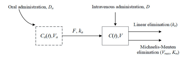
This study examined a single-compartment pharmacokinetic model with intravenous and oral administration. It investigated the trends in steady-state drug exposure and average steady-state plasma drug concentration under multiple dosing regimens. First, the combined drug administration model was a non-autonomous system, and we approximated the solution of the model by estimating the exact upper and lower bounds in conjunction with the comparison theorem for differential equations. We also demonstrated the existence, uniqueness, and stability of the solution. Second, we derived the steady-state drug exposure and compared it with the solution of the intravenous drug delivery model alone. The results indicate that the combined drug delivery scheme offers superior performance. Finally, we theoretically proved the change rule of average steady-state blood drug concentration under different dosing regimens, and verified its feasibility and rationality by combining the numerical simulation results of Phenytoin sodium.

Keywords:

Citation: Jiali Shi, Zhongyi Xiang. Mathematical analysis of nonlinear combination drug delivery[J]. Electronic Research Archive, 2025, 33(3): 1812-1835. doi: 10.3934/era.2025082

Related Papers:

[1]	Latifah Hanum, Dwi Ertiningsih, Nanang Susyanto . Sensitivity analysis unveils the interplay of drug-sensitive and drug-resistant Glioma cells: Implications of chemotherapy and anti-angiogenic therapy. Electronic Research Archive, 2024, 32(1): 72-89. doi: 10.3934/era.2024004
[2]	Ziang Chen, Chunguang Dai, Lei Shi, Gaofang Chen, Peng Wu, Liping Wang . Reaction-diffusion model of HIV infection of two target cells under optimal control strategy. Electronic Research Archive, 2024, 32(6): 4129-4163. doi: 10.3934/era.2024186
[3]	Yineng Ouyang, Zhaotao Liang, Zhihui Ma, Lei Wang, Zhaohua Gong, Jun Xie, Kuikui Gao . A class of constrained optimal control problems arising in an immunotherapy cancer remission process. Electronic Research Archive, 2024, 32(10): 5868-5888. doi: 10.3934/era.2024271
[4]	Qing Li, Junfeng He . Pattern formation in a ratio-dependent predator-prey model with cross diffusion. Electronic Research Archive, 2023, 31(2): 1106-1118. doi: 10.3934/era.2023055
[5]	Xianjun Wang, Huaguang Gu, Bo Lu . Big homoclinic orbit bifurcation underlying post-inhibitory rebound spike and a novel threshold curve of a neuron. Electronic Research Archive, 2021, 29(5): 2987-3015. doi: 10.3934/era.2021023
[6]	Jianmin Hou, Quansheng Liu, Hongwei Yang, Lixin Wang, Yuanhong Bi . Stability and bifurcation analyses of p53 gene regulatory network with time delay. Electronic Research Archive, 2022, 30(3): 850-873. doi: 10.3934/era.2022045
[7]	Xian Tan, Shijie Fan, Kaiwen Duan, Mengyue Xu, Jingbo Zhang, Pingping Sun, Zhiqiang Ma . A novel drug-drug interactions prediction method based on a graph attention network. Electronic Research Archive, 2023, 31(9): 5632-5648. doi: 10.3934/era.2023286
[8]	Xiaojun Huang, Zigen Song, Jian Xu . Amplitude death, oscillation death, and stable coexistence in a pair of VDP oscillators with direct–indirect coupling. Electronic Research Archive, 2023, 31(11): 6964-6981. doi: 10.3934/era.2023353
[9]	Fang Yan, Changyong Dai, Haihong Liu . Oscillatory dynamics of p53 pathway in etoposide sensitive and resistant cell lines. Electronic Research Archive, 2022, 30(6): 2075-2108. doi: 10.3934/era.2022105
[10]	Cunbin An . Global bifurcation and structure of stationary patterns of a diffusive system of plant-herbivore interactions with toxin-determined functional responses. Electronic Research Archive, 2023, 31(4): 2095-2107. doi: 10.3934/era.2023107

Abstract

1. Introduction

Pharmacokinetics (PK) focuses on the absorption, distribution, metabolism, and processes of drugs in the organism. By monitoring changes in the concentration of a drug in the plasma, researchers are able to describe these dynamic processes with the help of mathematical models, which allow them to make predictions about the disposition of the drug ^[1,2]. The use of mathematical models is particularly important in drugs because it provides a scientific tool to speculate on the in vivo behavior of a drug candidate based on a small amount of experimental data. The compartmental Model (CM) is one of the most commonly used PK models in drug studies and processes, and linear atrial models are the most common ^[3,4]. Many nonlinear and physiologically based pharmacokinetic models have also been derived in recent years, and the elimination pathways may include both first-order and Michaelis-Menten elimination ^[5,6,7]. They enable more accurate prediction of complex pharmacokinetic behaviors and assessment of the therapeutic effects of drugs. The emergence of these models provides a more accurate tool for drug discovery and development, helping to screen potential drug candidates at the preclinical stage and to predict their pharmacokinetic performance in humans.

In order to better understand the qualitative and quantitative behavior of drugs in vivo, the study of analytical solutions of pharmacokinetic models has received academic attention ^[8,9]. Tang and Xiao developed a one-compartment model with Michaelis-Menten elimination and a therapeutic window. They used the Lambert $W$ transcendental function to derive the analytical solution of the model under three different input conditions, designing a dosing regimen to ensure that the drug concentration remains within the therapeutic window ^[10]. Single-compartment and two-compartment fractional-order pharmacokinetic models have been studied by Dokoumetzidis and Sopasakis et al. They allowed the formulation of multicompartment models with consistent mixing of different fractional orders, and also provided a numerical inverse Laplace transform algorithm-based solution ^[11]. Wu et al. introduced a new $X$ transcendental function and provided the solution for a single-compartment pharmacokinetic model with parallel first-order and Michaelis-Menten elimination pathways. They also analyzed the dominant roles of the two elimination pathways under specific conditions. Building on this model, Wu further incorporated a constant endogenous production and investigated the case of multiple intravenous administrations, discussing the area under the curve and the average concentration at steady state ^[12,13]. Daryakenari et al. proposed the Al-Aristotle frameworks and CMINNs, which combine pharmacokinetic compartment models with gray-box identification and neural network methods. The aim is to leverage the strengths of both biophysical models and data-driven approaches to enhance the accuracy and predictive power of pharmacokinetic models ^[14,15].

With the biomedical technology, co-administration of drugs has gradually become an important strategy to improve therapeutic effects. In co-administration, two or more drugs are usually used in combination in the hope that, through drug-drug interactions, therapeutic effects that are difficult to achieve with a single drug can be achieved. Panaccione et al. compared the efficacy and safety of infliximab alone, azathioprine alone, and their combination in treating ulcerative colitis in a study involving 239 patients ^[16]. They concluded that combination therapy led to significantly better mucosal healing than azathioprine monotherapy. Maruthur N. M. evaluated the comparative effectiveness and safety of monotherapy versus selected metformin-based combination therapies in adults with type 2 diabetes ^[17]. Given metformin's beneficial effects on hemoglobin ${A_{1c}},$ weight, and cardiovascular mortality (compared to sulfonylureas), along with its relative safety, metformin is recommended as the first-line therapy for managing type 2 diabetes in adults. Apatinib and gefitinib were proposed as a co-administration regimen for the treatment of non-small-cell lung cancer (NSCLC) ^[18], and their pharmacokinetics and drug-drug interactions were investigated in the context of intravenous and oral administration. The results showed that co-administration can alter drug levels and metabolic pathways, which is important for optimizing treatment regimens. Hanum and colleagues studied glioma growth models using chemotherapy and anti-angiogenesis therapy ^[19]. Chemotherapy can lead to the emergence of resistant cells, while anti-angiogenesis therapy mitigates mutations by blocking nutrient delivery to tumor cells through the blood vessels. As a result, the combination of these two therapies achieves the best therapeutic outcomes.

However, the complexity of combining different drugs may pose problems such as drug-drug interactions and difficulty in dosage adjustment, prompting researchers to explore more simplified and precise treatment strategies ^[20,21]. Combining the same drug with several delivery methods has drawn interest recently as a cutting-edge therapeutic strategy. This approach is usually applied in the transition between acute and long-term treatment, where optimization of drug efficacy and minimization of toxic side effects are achieved by combining the pharmacokinetic characteristics of drugs under different modes of administration. Common modes of administration are intravenous, oral, intramuscular, and subcutaneous. With an intravenous injection (IV), the drug can enter the bloodstream directly, quickly reach the therapeutic concentration, avoid the liver and gastrointestinal tract's first-pass effect, and have a high bioavailability ^[22]. On the other hand, prolonged IV is prone to local circulatory disorders that lead to tissue hypoxia, resulting in side effects such as edema and phlebitis. The benefit of oral administration (PO) is that it is less expensive and allows patients to self-administer the drug at home without the need for specialized handling or equipment ^[23]. However, oral drug delivery have low bioavailability and variable absorption and efficacy. Additionally, patients may use drugs incorrectly or forget to take them, which would reduce the effectiveness of treatment. Compared to subcutaneous injections, intramuscular injections absorb the drug more quickly and are suitable for administering relatively large doses ^[24]. Nevertheless, this method of drug delivery may cause more pain. Subcutaneous injections are more appropriate for long-term treatments such as insulin injections and vaccinations. But its limitations include a restriction on the injection volume and a slower absorption rate. In this paper, we combine intravenous injection and oral administration, which can enhance one another's strengths. Despite the potential advantages, there is not much research on this dosing strategy. Kerin et al. compared amiodarone combined intravenous and oral dosing regimens with oral dosing alone and found that the combined regimen decreased the cumulative dose needed and shortened the time to achieve optimal ventricular arrhythmia control ^[25]. However, this literature was based on specific experimental studies and did not address the discussion of mathematical modeling. Therefore, using the previously stated mathematical model, we propose a new co-administration treatment regimen to explain the pharmacokinetic process.

This paper is organized as follows. In Section 2, we present a single-compartment PK model for intravenous combined oral administration. In Section 3, we give an exact approximate solution of the model, as well as proving the existence uniqueness and local stability of the solution. In Section 4, the steady-state drug exposure is calculated. Numerical simulations are used to compare the changes in plasma drug concentration and drug exposure between combination therapy and monotherapy, thereby evaluating the advantages of combination therapy. Section 5 derives the average steady-state concentration of the model and reveals the variation patterns of this key pharmacokinetic parameter under different dosing regimens. Section 6 demonstrates the practical application of the above patterns of change in conjunction with an example of a real drug. The final section discusses the limitations and prospects of the current work.

2. PK model of combined administration

Intravenous injection allows the drug to enter the systemic circulation directly, whereas oral administration requires an absorption phase before entering systemic circulation. The schematic diagram is shown in . Therefore, we focus only on their actions within the central compartment. Initially, an intravenous dose of ${D}$ is administered to achieve a specific blood concentration level, followed by an oral dose of ${D_a}$ . After an interval $\tau$ , another dose is administered. A single-compartment model for nonlinear oral combined IV drug administration is established based on this process as follows:

$\begin{eqnarray} \begin{array}{lll} \left\{ \begin{array}{lll} \frac{{d{C_a}\left( t \right)}}{{dt}} = - {k_a}{C_a}\left( t \right), {\kern 1pt} {\kern 1pt} {\kern 1pt} {\kern 1pt} t \ne n\tau , \\ {C_a}\left( {{t^ + }} \right) = {C_a}\left( t \right) + \frac{{{D_a}}}{{{V_a}}}, {\kern 1pt} {\kern 1pt} {\kern 1pt} {\kern 1pt} t = n\tau , \\ \frac{{d{C}\left( t \right)}}{{dt}} = F{k_a}{C_a}\left( t \right) - {k_e}{C}\left( t \right) - \frac{{{V_{\max }}{C}\left( t \right)}}{{{K_m} + {C}\left( t \right)}}, \ t \ne n\tau , \\ {C}\left( {{t^ + }} \right) = {C}\left( t \right) + \frac{{{D}}}{{{V}}}, \ t = n\tau , n = 0, 1, 2, \cdots \\ \end{array}\right. \end{array} \end{eqnarray}$

(2.1)

Figure 1. Single-compartment model for nonlinear combined oral and intravenous administration.

${C_a}\left(t \right)$ is the drug concentration in the peripheral compartment;

${C}\left(t \right)$ is the drug concentration in the central compartment;

${k_a}$ is the elimination rate of the drug in the peripheral compartment;

${k_e}$ is the elimination rate in the central compartment;

${V_{\max }}$ is the theoretical maximum rate of the process;

${K_m}$ is the Michaelis-Menten constant;

$F$ denotes the bioavailability of the drug transferring from the peripheral compartment to the central compartment; and

${V_a}$ and

${V}$ are the apparent volumes of distribution in the peripheral and central compartments, respectively.

DownLoad: Full-Size Img PowerPoint

3. Model solution

Model (2.1) can be viewed as the coupling of two PK systems: the peripheral compartment and the central compartment. The change in drug concentration in the peripheral compartment can be described as follows:

(3.1)

To find the solution of model (3.1) over the interval $t \in \left({n\tau, \left({n + 1} \right)\tau } \right],$ we proceed as follows:

${C_a}\left( t \right) = {C_a}\left( {n{\tau ^ + }} \right){e^{ - {k_a}\left( {t - n\tau } \right)}}.$

When $t = \left({n + 1} \right)\tau,$ the concentration at this time is

${C_a}\left( {\left( {n + 1} \right)\tau } \right) = {C_a}\left( {n{\tau ^ + }} \right){e^{ - {k_a}\tau }}.$

Moreover, we have

${C_a}\left( {\left( {n + 1} \right){\tau ^ + }} \right) = {C_a}\left( {\left( {n + 1} \right)\tau } \right) + \frac{{{D_a}}}{{{V_a}}} = {C_a}\left( {n{\tau ^ + }} \right){e^{ - {k_a}\tau }} + \frac{{{D_a}}}{{{V_a}}}.$

Since ${e^{ - {k_a}\tau }} < 1,$ the equation has a stable fixed point given by

$x_a^* = \frac{{{D_a}}}{{{V_a}\left( {1 - {e^{ - {k_a}\tau }}} \right)}}.$

Substituting the fixed point into the solution of Eq (3.1), we obtain a stable periodic solution as

${\tilde C_a}\left( t \right){\kern 1pt} = x_a^*{e^{ - {k_a}\left( {t - n\tau } \right)}} = \frac{{{D_a}}}{{{V_a}\left( {1 - {e^{ - {k_a}\tau }}} \right)}}{e^{ - {k_a}\left( {t - n\tau } \right)}}, t \in \left( {n\tau , \left( {n + 1} \right)\tau } \right].$

The following discusses the changes in drug concentration in the central compartment when the absorption compartment is in a steady state.

$\begin{eqnarray} \begin{array}{lll} \left\{ \begin{array}{lll} \frac{{d{C}\left( t \right)}}{{dt}} = F{k_a}{C_a}\left( t \right) - {k_e}{C}\left( t \right) - \frac{{{V_{\max }}{C}\left( t \right)}}{{{K_m} + {C}\left( t \right)}}, \ t \ne n\tau , \\ {C}\left( {{t^ + }} \right) = {C}\left( t \right) + \frac{{{D}}}{{{V}}}, \ t = n\tau . \\ \end{array}\right. \end{array} \end{eqnarray}$

(3.2)

By directly substituting the steady-state solution of the peripheral compartment into the model, the first equation of model (3.2) becomes

$\begin{array}{l} \frac{{dC\left( t \right)}}{{dt}} = F{k_a}\frac{{{D_a}}}{{{V_a}\left( {1 - {e^{ - {k_a}\tau }}} \right)}}{e^{ - {k_a}\left( {t - n\tau } \right)}} - {k_e}C\left( t \right) - \frac{{{V_{\max }}C\left( t \right)}}{{{K_m} + C\left( t \right)}} \\ {\kern 1pt} {\kern 1pt} {\kern 1pt} {\kern 1pt} {\kern 1pt} {\kern 1pt} {\kern 1pt} {\kern 1pt} {\kern 1pt} {\kern 1pt} {\kern 1pt} {\kern 1pt} {\kern 1pt} {\kern 1pt} {\kern 1pt} {\kern 1pt} {\kern 1pt} {\kern 1pt} {\kern 1pt} {\kern 1pt} {\kern 1pt} {\kern 1pt} {\kern 1pt} = f\left( \tau \right) \cdot {e^{ - {k_a}t}} - {k_e}C\left( t \right) - \frac{{{V_{\max }}C\left( t \right)}}{{{K_m} + C\left( t \right)}}, \\ \end{array}$

where $f\left(\tau \right) = \frac{{F{k_a}{D_a}}}{{{V_a}\left({1 - {e^{ - {k_a}\tau }}} \right)}}{e^{{k_a}n\tau }}.$ Then the model is transformed into

$\begin{eqnarray} \begin{array}{lll} \left\{ \begin{array}{lll} \frac{{d{C}\left( t \right)}}{{dt}} = f\left( \tau \right){e^{ - {k_a}t}} - {k_e}{C}\left( t \right) - \frac{{{V_{\max }}{C}\left( t \right)}}{{{K_m} + {C}\left( t \right)}}, \ t \ne n\tau, \\ {C}\left( {{t^ + }} \right) = {C}\left( t \right) + \frac{{{D}}}{{{V}}}, \ t = n\tau . \\ \end{array}\right. \end{array} \end{eqnarray}$

(3.3)

This is a non-autonomous first-order differential equation that cannot be directly solved analytically. Therefore, we seek the upper and lower bounds of model (3.3) on each interval, and then extend these bounds across the entire interval. By finding bounds in each sub-interval, we can approximate the behavior of the solution over $\left[{n\tau, \left({n + 1} \right)\tau } \right]$ , allowing us to construct an understanding of the solution's range and stability across the entire interval. This approach provides a framework for analyzing the solution behavior even when an explicit solution is unattainable.

3.1. Exact upper and lower bounds on the solution

We are primarily interested in the steady-state situation following the periodic administration of the drug, with the system's changes occurring mainly at the moments of administration and cessation. To simplify the problem, we can focus solely on the states at the beginning and end of each cycle. Specifically, we consider the two endpoints of the interval, construct two subsystems, and label the corresponding solutions. This approach effectively simplifies the non-autonomous system by discretizing time ^[26]. Therefore, we apply the comparison theorem for differential equations, a mathematical tool used to analyze upper and lower bounds on solutions. It is often employed to study the growth, convergence, and uniqueness of solutions to differential equations. If a function satisfies a certain differential inequality, its solution can be governed by another known function. We denote ${C_{low}}\left(t \right)$ and ${C_{up}}\left(t \right)$ as the solutions of the following two models:

$\begin{array}{c}\frac{{d{C_{low}}\left( t \right)}}{{dt}} = f\left( \tau \right){e^{ - {k_a}\left( {n + 1} \right)\tau }} - {k_e}{C_{low}}\left( t \right) - \frac{{{V_{\max }}{C_{low}}\left( t \right)}}{{{K_m} + {C_{low}}\left( t \right)}}, \\ \frac{{d{C_{up}}\left( t \right)}}{{dt}} = f\left( \tau \right){e^{ - {k_a}n\tau }} - {k_e}{C_{up}}\left( t \right) - \frac{{{V_{\max }}{C_{up}}\left( t \right)}}{{{K_m} + {C_{up}}\left( t \right)}}. \end{array}$

For model (3.3), it can be observed that

$\begin{eqnarray} \begin{array}{lll} f\left( \tau \right){e^{ - {k_a}\left( {n + 1} \right)\tau }} \le f\left( \tau \right){e^{ - {k_a}t}} \le f\left( \tau \right){e^{ - {k_a}n\tau }} \end{array} \end{eqnarray}$

(3.4)

for $t \in \left[{n\tau, \left({n + 1} \right)\tau } \right]$ . According to the comparison theorem for differential equations, the solution $C\left(t \right)$ of model (3.3) satisfies ${C_{low}}\left(t \right) \le C\left(t \right) \le {C_{up}}\left(t \right).$

First, we have to find the exact upper bound. If $t = n\tau$ , then Eq (3.3) becomes

$\begin{eqnarray} \begin{array}{lll} \left\{ \begin{array}{lll} \frac{{d{C_{up}}\left( t \right)}}{{dt}} = \sigma - {k_e}{C_{up}}\left( t \right) - \frac{{{V_{\max }}{C_{up}}\left( t \right)}}{{{K_m} + {C_{up}}\left( t \right)}}, \ t \ne n\tau , \\ {C_{up}}\left( {{t^ + }} \right) = {C_{up}}\left( t \right) + \frac{{{D}}}{{{V}}}, \ t = n\tau , \\ \end{array}\right. \end{array} \end{eqnarray}$

(3.5)

where $\sigma = f\left(\tau \right){e^{ - {k_a}n\tau }} = F{k_a}x_a^*$ . Divide both sides of the first equation by ${k_e}{C_{up}}\left(t \right)$ :

${\kern 1pt} \frac{{\left( {1/{k_e}} \right)\left( {{K_m} + {C_{up}}\left( t \right)} \right)}}{{{C_{up}}^2\left( t \right) + \left( {{K_m} + {V_{\max }}/{k_e} - \sigma/{k_e}} \right){C_{up}}\left( t \right) - {K_m}\sigma/{k_e}}}d{C_{up}}\left( t \right) = - dt.$

Rearrange the above equation as

$\begin{eqnarray} \begin{array}{lll} \left( {\frac{p}{{{C_{up}}\left( t \right) - \alpha }} + \frac{q}{{{C_{up}}\left( t \right) + \beta }}} \right)d{C_{up}}\left( t \right) = - dt, \end{array} \end{eqnarray}$

(3.6)

where $p = \frac{{{K_m} + \alpha }}{{{k_e}\left({\alpha + \beta } \right)}}$ , $q = \frac{{\beta - {K_m}}}{{{k_e}\left({\alpha + \beta } \right)}}$ ,

$\begin{array}{c} \alpha = \frac{{2{K_m}\sigma}}{{{K_m}{k_e} + {V_{\max }} - \sigma + \sqrt {{{\left( {{K_m}{k_e} + {V_{\max }} - \sigma} \right)}^2} + 4{K_m}{k_e}\sigma} }}, \\ \beta = \frac{{{K_m}{k_e} + {V_{\max }} - \sigma + \sqrt {{{\left( {{K_m}{k_e} + {V_{\max }} - \sigma} \right)}^2} + 4{K_m}\sigma} }}{{2{k_e}}}. \end{array}$

At the same time, $p,$ $q,$ $\alpha$ , and $\beta$ are positive. Integrating Eq (3.6) yields

${\left( {{C_{up}}\left( t \right) - \alpha } \right)^p}{\left( {{C_{up}}\left( t \right) + \beta } \right)^q} = {\left( {{C_{up}}\left( {n{\tau ^ + }} \right) - \alpha } \right)^p}{\left( {{C_{up}}\left( {n{\tau ^ + }} \right) + \beta } \right)^q}{e^{ - \left( {t - n\tau } \right)}}.$

Divide both sides by ${\left({\alpha + \beta } \right)^{p + q}}$ and further write it as

${\left( {\frac{{{C_{up}}\left( t \right) - \alpha }}{{\alpha + \beta }}} \right)^p}{\left( {\frac{{{C_{up}}\left( t \right) - \alpha }}{{\alpha + \beta }} + 1} \right)^q} = {\left( {\frac{{{C_{up}}\left( {n{\tau ^ + }} \right) - \alpha }}{{\alpha + \beta }}} \right)^p}{\left( {\frac{{{C_{up}}\left( {n{\tau ^ + }} \right) + \beta }}{{\alpha + \beta }}} \right)^q}{e^{ - \left( {t - n\tau } \right)}}.$

Definition 1 (See ^[12]) We define X as the solution of the following equation:

$X{\left( {z, p, q} \right)^p}{\left( {X\left( {z, p, q} \right) + 1} \right)^q} = z,$

where $p, q \in {\mathbb{R}^ + }$ , and $z$ is a complex number.

According to the definition of the $X$ function, $\frac{{{C_{up}}\left(t \right) - \alpha }}{{\alpha + \beta }}$ can be written as

$\frac{{{C_{up}}\left( t \right) - \alpha }}{{\alpha + \beta }} = X\left( {{{\left( {\frac{{{C_{up}}\left( {n{\tau ^ + }} \right) - \alpha }}{{\alpha + \beta }}} \right)}^p}{{\left( {\frac{{{C_{up}}\left( {n{\tau ^ + }} \right) + \beta }}{{\alpha + \beta }}} \right)}^q}{e^{ - \left( {t - n\tau } \right)}}, p, q} \right).$

Hence any solution of model (3.5) is

$\begin{eqnarray} \begin{array}{lll} {C_{up}}\left( t \right) = \alpha + \left( {\alpha + \beta } \right) \cdot X\left( {{{\left( {\frac{{{C_{up}}\left( {n\tau } \right) + {D}/{V} - \alpha }}{{\alpha + \beta }}} \right)}^p}} \right. \\ \left. {{\kern 1pt} {\kern 1pt} {\kern 1pt} {\kern 1pt} {\kern 1pt} {\kern 1pt} {\kern 1pt} {\kern 1pt} {\kern 1pt} {\kern 1pt} {\kern 1pt} {\kern 1pt} {\kern 1pt} {\kern 1pt} {\kern 1pt} {\kern 1pt} {\kern 1pt} {\kern 1pt} {\kern 1pt} {\kern 1pt} {\kern 1pt} {\kern 1pt} {\kern 1pt} {\kern 1pt} {\kern 1pt} {\kern 1pt} {\kern 1pt} {\kern 1pt} {\kern 1pt} {\kern 1pt} {\kern 1pt} {\kern 1pt} {\kern 1pt} {\kern 1pt} {\kern 1pt} {\kern 1pt} {{\left( {\frac{{{C_{up}}\left( {n\tau } \right) + {D}/{V} + \beta }}{{\alpha + \beta }}} \right)}^q}{e^{ - \left( {t - n\tau } \right)}}, p, q} \right). \\ \end{array} \end{eqnarray}$

(3.7)

In particular,

$\begin{eqnarray} \begin{array}{lll} {C_{up}}\left( {\left( {n + 1} \right)\tau } \right) = \alpha + \left( {\alpha + \beta } \right) \cdot X\left( {{{\left( {\frac{{{C_{up}}\left( {n\tau } \right) + {D}/{V} - \alpha }}{{\alpha + \beta }}} \right)}^p}} \right. \\ \left. {{\kern 1pt} {\kern 1pt} {\kern 1pt} {\kern 1pt} {\kern 1pt} {\kern 1pt} {\kern 1pt} {\kern 1pt} {\kern 1pt} {\kern 1pt} {\kern 1pt} {\kern 1pt} {\kern 1pt} {\kern 1pt} {\kern 1pt} {\kern 1pt} {\kern 1pt} {\kern 1pt} {\kern 1pt} {\kern 1pt} {\kern 1pt} {\kern 1pt} {\kern 1pt} {\kern 1pt} {\kern 1pt} {\kern 1pt} {\kern 1pt} {\kern 1pt} {\kern 1pt} {\kern 1pt} {\kern 1pt} {\kern 1pt} {\kern 1pt} {\kern 1pt} {\kern 1pt} {\kern 1pt} {\kern 1pt} {\kern 1pt} {\kern 1pt} {\kern 1pt} {\kern 1pt} {\kern 1pt} {\kern 1pt} {\kern 1pt} {\kern 1pt} {\kern 1pt} {\kern 1pt} {\kern 1pt} {\kern 1pt} {\kern 1pt} {\kern 1pt} {\kern 1pt} {\kern 1pt} {\kern 1pt} {\kern 1pt} {\kern 1pt} {\kern 1pt} {\kern 1pt} {\kern 1pt} {\kern 1pt} {\kern 1pt} {\kern 1pt} {\kern 1pt} {\kern 1pt} {\kern 1pt} {\kern 1pt} {\kern 1pt} {\kern 1pt} {\kern 1pt} {\kern 1pt} {{\left( {\frac{{{C_{up}}\left( {n\tau } \right) + {D}/{V} + \beta }}{{\alpha + \beta }}} \right)}^q}{e^{ - \tau }}, p, q} \right), \\ \end{array} \end{eqnarray}$

(3.8)

$\begin{eqnarray} \begin{array}{lll} {C_{up}}\left( {{{\left( {n + 1} \right)}^ + }\tau } \right) = \alpha + \left( {\alpha + \beta } \right) \cdot X\left( {{{\left( {\frac{{{C_{up}}\left( {n\tau } \right) + {D}/{V} - \alpha }}{{\alpha + \beta }}} \right)}^p}} \right. \\ \left. {{\kern 1pt} {\kern 1pt} {\kern 1pt} {\kern 1pt} {\kern 1pt} {\kern 1pt} {\kern 1pt} {\kern 1pt} {\kern 1pt} {\kern 1pt} {\kern 1pt} {\kern 1pt} {\kern 1pt} {\kern 1pt} {\kern 1pt} {\kern 1pt} {\kern 1pt} {\kern 1pt} {\kern 1pt} {\kern 1pt} {\kern 1pt} {\kern 1pt} {\kern 1pt} {\kern 1pt} {\kern 1pt} {\kern 1pt} {\kern 1pt} {\kern 1pt} {\kern 1pt} {\kern 1pt} {\kern 1pt} {\kern 1pt} {\kern 1pt} {\kern 1pt} {\kern 1pt} {\kern 1pt} {\kern 1pt} {\kern 1pt} {\kern 1pt} {\kern 1pt} {\kern 1pt} {\kern 1pt} {\kern 1pt} {\kern 1pt} {\kern 1pt} {\kern 1pt} {\kern 1pt} {\kern 1pt} {\kern 1pt} {\kern 1pt} {\kern 1pt} {\kern 1pt} {\kern 1pt} {\kern 1pt} {\kern 1pt} {\kern 1pt} {\kern 1pt} {\kern 1pt} {\kern 1pt} {\kern 1pt} {\kern 1pt} {\kern 1pt} {\kern 1pt} {\kern 1pt} {\kern 1pt} {\kern 1pt} {\kern 1pt} {\kern 1pt} {\kern 1pt} {\kern 1pt} {{\left( {\frac{{{C_{up}}\left( {n\tau } \right) + {D}/{V} + \beta }}{{\alpha + \beta }}} \right)}^q}{e^{ - \tau }}, p, q} \right) + \frac{{{D}}}{{{V}}}. \\ \end{array} \end{eqnarray}$

(3.9)

To determine the steady-state concentration at any given time $t$ , we define ${C_n} = {C_{up}}\left({n\tau } \right)$ . Hence Eq (3.8) becomes

$\begin{eqnarray} \begin{array}{lll} {C_{n + 1}}{\kern 1pt} = \alpha + \left( {\alpha + \beta } \right) \cdot X\left( {{{\left( {\frac{{{C_n} + {D}/{V} - \alpha }}{{\alpha + \beta }}} \right)}^p}{{\left( {\frac{{{C_n} + {D}/{V} + \beta }}{{\alpha + \beta }}} \right)}^q}{e^{ - \tau }}, p, q} \right). \end{array} \end{eqnarray}$

(3.10)

Using the definition of the $X$ function, the above equation is rearranged as

$\begin{eqnarray} \begin{array}{lll} {\left( {\frac{{{C_{n + 1}} - \alpha }}{{{C_n} + {D}/{V} - \alpha }}} \right)^{1 - r}}{\left( {\frac{{{C_{n + 1}} + \beta }}{{{C_n} + {D}/{V} + \beta }}} \right)^r} = {e^{ - {k_e}\tau }}, \end{array} \end{eqnarray}$

(3.11)

where $r = \frac{{\beta - {K_m}}}{{\alpha + \beta }} \in \left({0, 1} \right),$ i.e., $\beta > {K_m}$ . Let the steady-state solution ${C^*} = {C_n} = {C_{n + 1}}$ , and we obtain

$\begin{eqnarray} \begin{array}{lll} {\left( {\frac{{{C^*} - \alpha }}{{{C^*} + {D}/{V} - \alpha }}} \right)^{1 - r}}{\left( {\frac{{{C^*} + \beta }}{{{C^*} + {D}/{V} + \beta }}} \right)^r} = {e^{ - {k_e}\tau }}. \end{array} \end{eqnarray}$

(3.12)

We know that ${C^*}$ uniquely exists (the proof of the existence and uniqueness is given in the next subsection), and thus we get the unique periodic solution as

$\begin{eqnarray} \begin{array}{lll} {{\tilde C}_{up}}\left( t \right) = \alpha + \left( {\alpha + \beta } \right) \cdot X\left( {{{\left( {\frac{{{C^*} + {D}/{V} - \alpha }}{{\alpha + \beta }}} \right)}^p}} \right. \\ \left. {{\kern 1pt} {\kern 1pt} {\kern 1pt} {\kern 1pt} {\kern 1pt} {\kern 1pt} {\kern 1pt} {\kern 1pt} {\kern 1pt} {\kern 1pt} {\kern 1pt} {\kern 1pt} {\kern 1pt} {\kern 1pt} {\kern 1pt} {\kern 1pt} {\kern 1pt} {\kern 1pt} {\kern 1pt} {\kern 1pt} {\kern 1pt} {\kern 1pt} {\kern 1pt} {\kern 1pt} {\kern 1pt} {\kern 1pt} {\kern 1pt} {\kern 1pt} {\kern 1pt} {\kern 1pt} {\kern 1pt} {\kern 1pt} {\kern 1pt} {\kern 1pt} {\kern 1pt} {\kern 1pt} {\kern 1pt} {\kern 1pt} {\kern 1pt} {\kern 1pt} {\kern 1pt} {{\left( {\frac{{{C^*} + {D}/{V} + \beta }}{{\alpha + \beta }}} \right)}^q}{e^{ - \left( {t - n\tau } \right)}}, p, q} \right), {\kern 1pt} {\kern 1pt} {\kern 1pt} {\kern 1pt} {\kern 1pt} {\kern 1pt} t \in \left( {n\tau , \left( {n + 1} \right)\tau } \right]. \\ \end{array} \end{eqnarray}$

(3.13)

Now we seek the lower bound. If $t = \left({n + 1} \right)\tau$ , then Eq (3.3) becomes

$\left\{ \begin{array}{l} \frac{{d{C_{low}}\left( t \right)}}{{dt}} = \sigma {e^{ - {k_a}\tau }}- {k_e}{C_{low}}\left( t \right) - \frac{{{V_{\max }}{C_{low}}\left( t \right)}}{{{K_m} + {C_{low}}\left( t \right)}}, \ t \ne n\tau, \\ {C_{low}}\left( {{t^ + }} \right) = {C_{low}}\left( t \right) + \frac{{{D}}}{{{V}}}, \ t = n\tau , \\ \end{array} \right.$

where $\sigma {e^{ - {k_a}\tau }} = f\left(\tau \right){e^{ - {k_a}\left({n + 1} \right)\tau }} = F{k_a}x_a^*{e^{ - {k_a}\tau }}$ . Similarly, using the same approach, the solution of the model is given by

$\begin{array}{l} {{\tilde C}_{low}}\left( t \right) = {\alpha _1} + \left( {{\alpha _1} + {\beta _1}} \right) \cdot X\left( {{{\left( {\frac{{{C^*} + {D}/{V} - {\alpha _1}}}{{{\alpha _1} + {\beta _1}}}} \right)}^{p_1}}} \right. \\ \left. {{\kern 1pt} {\kern 1pt} {\kern 1pt} {\kern 1pt} {\kern 1pt} {\kern 1pt} {\kern 1pt} {\kern 1pt} {\kern 1pt} {\kern 1pt} {\kern 1pt} {\kern 1pt} {\kern 1pt} {\kern 1pt} {\kern 1pt} {\kern 1pt} {\kern 1pt} {\kern 1pt} {\kern 1pt} {\kern 1pt} {\kern 1pt} {\kern 1pt} {\kern 1pt} {\kern 1pt} {\kern 1pt} {\kern 1pt} {\kern 1pt} {\kern 1pt} {\kern 1pt} {\kern 1pt} {\kern 1pt} {\kern 1pt} {\kern 1pt} {\kern 1pt} {\kern 1pt} {\kern 1pt} {\kern 1pt} {\kern 1pt} {\kern 1pt} {\kern 1pt} {\kern 1pt} {{\left( {\frac{{{C^*} + {D}/{V} + {\beta _1}}}{{{\alpha _1} + {\beta _1}}}} \right)}^{q_1}}{e^{ - \left( {t - n\tau } \right)}}, {p_1}, {q_1}} \right), {\kern 1pt} {\kern 1pt} {\kern 1pt} {\kern 1pt} {\kern 1pt} {\kern 1pt} t \in \left( {n\tau , \left( {n + 1} \right)\tau } \right], \\ \end{array}$

where ${p_1} = \frac{{{K_m} + {\alpha _1}}}{{{k_e}\left({\alpha _1} + {\beta _1} \right)}},$ ${q_1} = \frac{{{\beta _1} - {K_m}}}{{{k_e}\left({{\alpha _1} + {\beta _1}} \right)}},$

$\begin{array}{c} {\alpha _1} = \frac{{2{K_m}\sigma {e^{ - {k_a}\tau }}}}{{{K_m}{k_e} + {V_{\max }} - \sigma {e^{ - {k_a}\tau }} + \sqrt {{{\left( {{K_m}{k_e} + {V_{\max }} - \sigma {e^{ - {k_a}\tau }}} \right)}^2} + 4{K_m}{k_e}\sigma {e^{ - {k_a}\tau }}} }}, \\ {\beta _1} = \frac{{{K_m}{k_e} + {V_{\max }} - \sigma {e^{ - {k_a}\tau }} + \sqrt {{{\left( {{K_m}{k_e} + {V_{\max }} - \sigma {e^{ - {k_a}\tau }}} \right)}^2} + 4{K_m}{k_e}\sigma {e^{ - {k_a}\tau }}} }}{{2{k_e}}}. \end{array}$

The exact upper and lower bounds of model (3.3) in each interval of length $\tau$ are derived separately according to the above method. Connect each interval by numerical simulation.

The concentrations exhibit periodic changes, as shown in Figure 2, and the upper and lower bounds steadily decrease and are consistent with the trend of the precise solution. In order to simplify the subsequent analysis, we choose upper bounds with very small differences from the exact solution for our study, which ensures accuracy and reduces computational complexity. This approach is commonly used to analyze complex periodic systems and can help us understand the range of up and down fluctuations in drug concentration especially in multiple dosing models.

Figure 2. Approximation between the exact solution and the upper and lower bounds.

$F = 0.8$ ;

${k_a} = 0.25/h$ ;

${k_e} = 0.21/h$ ;

${K_m} = 1.5mM$ ;

${V_{\max }} = 1.5mg/\min$ ;

${V_a} = 2L$ ;

${V} = 2L$ ;

${D_a} = 8mg$ ;

${D} = 4mg$ ;

$\tau = 4h$ .

DownLoad: Full-Size Img PowerPoint

For ease of writing, we replace ${\tilde C_{up}}\left(t \right)$ with ${\tilde C}\left(t \right)$ . According to Eq (3.13), the solution in the interval $\left({n\tau, \left({n + 1} \right)\tau } \right]$ is

$\begin{eqnarray} \begin{array}{lll} \tilde C\left( t \right) = \alpha + \left( {\alpha + \beta } \right) \cdot X\left( {{{\left( {\frac{{{C^*} + D/V - \alpha }}{{\alpha + \beta }}} \right)}^p}} \right.\left. {{{\left( {\frac{{{C^*} + D/V + \beta }}{{\alpha + \beta }}} \right)}^q}{e^{ - \left( {t - n\tau } \right)}}, p, q} \right). \end{array} \end{eqnarray}$

(3.14)

The minimum steady-state blood drug concentration is

${\tilde C_{\min }} = \alpha + \left( {\alpha + \beta } \right) \cdot X\left( {{{\left( {\frac{{{C^*} + D/V - \alpha }}{{\alpha + \beta }}} \right)}^p}{{\left( {\frac{{{C^*} + D/V + \beta }}{{\alpha + \beta }}} \right)}^q}{e^{ - \tau }}, p, q} \right),$

and the maximum steady-state blood drug concentration is

${\tilde C_{\max }} = \alpha + \left( {\alpha + \beta } \right) \cdot X\left( {{{\left( {\frac{{{C^*} + D/V - \alpha }}{{\alpha + \beta }}} \right)}^p}{{\left( {\frac{{{C^*} + D/V + \beta }}{{\alpha + \beta }}} \right)}^q}{e^{ - \tau }}, p, q} \right) + \frac{D}{V}.$

3.2. Existence uniqueness and local stability analysis of the periodic solution

The existence and uniqueness of the periodic solution is the basis for analyzing the periodic behavior of the system, and the local stability further portrays the behavior of the system in response to the perturbation of the periodic solution. The ability of the system to sustain a specific periodic state, such as the preservation of stable fluctuations in drug concentration, is determined by the stability of the periodic solution. As a result, the study of these two properties offers methodological direction for real-world applications in the domains of pharmacokinetics in addition to theoretical significance.

Theorem 2 The periodic solution given by Eq (3.14) exists uniquely.

Proof. Define the left-hand side of Eq (3.12) as a function $F\left({{C^*}} \right)$ , i.e.,

$F\left( {{C^*}} \right) = {\left( {\frac{{{C^*} - \alpha }}{{{C^*} + D/V - \alpha }}} \right)^{1 - r}}{\left( {\frac{{{C^*} + \beta }}{{{C^*} + D/V + \beta }}} \right)^r}.$

The solution ${C^*}$ of $F\left({{C^*}} \right) = {e^{ - {k_e}\tau }}$ must be shown to be unique in an equivalent way in order to demonstrate the uniqueness of the periodic solution. The derivatives of the following expressions are all greater than 0, namely,

$\begin{array}{c}\frac{d}{{d{C^*}}}\left( {\frac{{{C^*} - \alpha }}{{{C^*} + D/V - \alpha }}} \right) = \frac{{D/V}}{{{{\left( {{C^*} + D/V - \alpha } \right)}^2}}} > 0, \\ \frac{d}{{d{C^*}}}\left( {\frac{{{C^*} + \beta }}{{{C^*} + D/V + \beta }}} \right) = \frac{{D/V}}{{{{\left( {{C^*} + D/V + \beta } \right)}^2}}} > 0.\end{array}$

Hence $F\left({{C^*}} \right)$ is globally rising as it is the product of these two partially increasing functions and the powers $1 - r$ and $r$ are both positive. This means that $F\left({{C^*}} \right)$ has at most one point of intersection with ${e^{ - {k_e}\tau }}$ , as shown in . Consequently, there is only one solution to the equation $F\left({{C^*}} \right) = {e^{ - {k_e}\tau }}$ . At the same time, we deduce that

$F\left( 0 \right) = {\left( {\frac{{ - \alpha }}{{D/V - \alpha }}} \right)^{1 - r}}{\left( {\frac{\beta }{{D/V + \beta }}} \right)^r} < 0, {\kern 1pt} {\kern 1pt} {\kern 1pt} {\kern 1pt} {\kern 1pt} {\kern 1pt} {\kern 1pt} \mathop {\lim }\limits_{{C^*} \to + \infty } F\left( {{C^*}} \right) = 1.$

Thus the continuity theorem requires that a solution ${C^*}$ exists for ${e^{ - {k_e}\tau }} \in \left({0, 1} \right)$ . In conclusion, the solution ${C^*}$ to the equation $F\left({{C^*}} \right) = {e^{ - {k_e}\tau }}$ exists uniquely, i.e., the periodic solution exists uniquely.

Figure 3. Schematic representation of the uniqueness of the existence of

$C^*$ .

${k_e} = 0.21/h$ ;

${K_m} = 0.5mM$ ;

${V} = 1L$ ;

${D} = 4mg$ ;

$\tau = 2h$ .

DownLoad: Full-Size Img PowerPoint

Theorem 3 The periodic solution given by Eq (3.14) is locally stable if

Proof. Define

$g\left( {{C}\left( {n + 1} \right){\tau ^ + }} \right) = {\left( {\frac{{{C}\left( {n + 1} \right){\tau ^ + } - \alpha }}{{\alpha + \beta }}} \right)^p}{\left( {\frac{{{C}\left( {n + 1} \right){\tau ^ + } + \beta }}{{\alpha + \beta }}} \right)^q}{e^{ - \tau }}.$

Equation (3.9) is deformed into

$\begin{array}{l} C\left( {\left( {n + 1} \right){\tau ^ + }} \right){\kern 1pt} = \alpha + \left( {\alpha + \beta } \right) \cdot X\left( {g\left( {C\left( {n + 1} \right){\tau ^ + }} \right), p, q} \right) + D/V \\ {\kern 1pt} {\kern 1pt} {\kern 1pt} {\kern 1pt} {\kern 1pt} {\kern 1pt} {\kern 1pt} {\kern 1pt} {\kern 1pt} {\kern 1pt} {\kern 1pt} {\kern 1pt} {\kern 1pt} {\kern 1pt} {\kern 1pt} {\kern 1pt} {\kern 1pt} {\kern 1pt} {\kern 1pt} {\kern 1pt} {\kern 1pt} {\kern 1pt} {\kern 1pt} {\kern 1pt} {\kern 1pt} {\kern 1pt} {\kern 1pt} {\kern 1pt} {\kern 1pt} {\kern 1pt} {\kern 1pt} {\kern 1pt} {\kern 1pt} {\kern 1pt} {\kern 1pt} {\kern 1pt} {\kern 1pt} {\kern 1pt} {\kern 1pt} {\kern 1pt} {\kern 1pt} {\kern 1pt} {\kern 1pt} {\kern 1pt} {\kern 1pt} {\kern 1pt} {\kern 1pt} {\kern 1pt} {\kern 1pt} {\kern 1pt} {\kern 1pt} {\kern 1pt} {\kern 1pt} {\kern 1pt} {\kern 1pt} {\kern 1pt} {\kern 1pt} {\kern 1pt} {\kern 1pt} {\kern 1pt} {\kern 1pt} {\kern 1pt} {\kern 1pt} {\kern 1pt} {\kern 1pt} {\kern 1pt} {\kern 1pt} {\kern 1pt} {\kern 1pt} : = \Gamma \left( {C\left( {\left( {n + 1} \right){\tau ^ + }} \right)} \right). \\ \end{array}$

Clearly, ${\tilde C_{\max }}$ is an equilibrium point in the equation above. The above equation's derivation leads to

$\begin{eqnarray} \begin{array}{lll} \frac{{\partial \Gamma \left( {{C}\left( {\left( {n + 1} \right){\tau ^ + }} \right)} \right)}}{{\partial {C}\left( {\left( {n + 1} \right){\tau ^ + }} \right)}} = \left( {\alpha + \beta } \right)\frac{{\partial X}}{{\partial z}} \cdot \frac{{\partial g}}{{\partial {C}\left( {\left( {n + 1} \right){\tau ^ + }} \right)}}. \end{array} \end{eqnarray}$

(3.15)

Here $X\left({z, p, q} \right)$ is simply written as $X$ . We let $H = {X^p}{\left({X + 1} \right)^q} - z$ according to the specification of $X$ .

The following partial derivatives with respect to $z$ and $X$ are obtained separately for $H$ .

${H_z} = - 1,$

$\begin{array}{l} {H_X} = {X^{p - 1}}{\left( {X + 1} \right)^{q - 1}}\left( {p\left( {X + 1} \right) + qX} \right) \\ {\kern 1pt} {\kern 1pt} {\kern 1pt} {\kern 1pt} {\kern 1pt} {\kern 1pt} {\kern 1pt} {\kern 1pt} {\kern 1pt} {\kern 1pt} {\kern 1pt} {\kern 1pt} {\kern 1pt} {\kern 1pt} {\kern 1pt} {\kern 1pt} = {X^p}{\left( {X + 1} \right)^q}\left( {\frac{p}{X} + \frac{q}{{X + 1}}} \right) \\ {\kern 1pt} {\kern 1pt} {\kern 1pt} {\kern 1pt} {\kern 1pt} {\kern 1pt} {\kern 1pt} {\kern 1pt} {\kern 1pt} {\kern 1pt} {\kern 1pt} {\kern 1pt} {\kern 1pt} {\kern 1pt} {\kern 1pt} {\kern 1pt} = z\left( {\frac{p}{X} + \frac{q}{{X + 1}}} \right). \\ \end{array}$

This leads to

$\frac{{\partial X}}{{\partial z}} = - \frac{{{H_z}}}{{{H_X}}} = - \frac{{ - 1}}{{z\left( {\frac{p}{X} + \frac{q}{{X + 1}}} \right)}} = \frac{1}{z}{\left( {\frac{p}{X} + \frac{q}{{X + 1}}} \right)^{ - 1}}.$

At steady state, $X$ satisfies the following equation:

$X\left( {g\left( {{C}\left( {n + 1} \right){\tau ^ + }} \right), p, q} \right) = \frac{{{{\tilde C}_{\max }} - {D}/{V} - \alpha }}{{\alpha + \beta }},$

and thus

$\frac{{\partial X}}{{\partial z}} = \frac{1}{z} \cdot \frac{1}{{\alpha + \beta }}{\left( {\frac{p}{{{{\tilde C}_{\max }} - {D}/{V} - \alpha }} + \frac{q}{{{{\tilde C}_{\max }} - {D}/{V} + \beta }}} \right)^{ - 1}}.$

At the same time, we calculate that the partial derivative of the function $g$ as

$\begin{array}{l} {\left. {\frac{{\partial g}}{{\partial {C}\left( {\left( {n + 1} \right){\tau ^ + }} \right)}}} \right|_{{C}\left( {\left( {n + 1} \right){\tau ^ + }} \right) = {{\tilde C}_{\max }}}} = \left( {\frac{p}{{{C}\left( {\left( {n + 1} \right){\tau ^ + }} \right) - \alpha }} + \frac{q}{{{C}\left( {\left( {n + 1} \right){\tau ^ + }} \right) + \beta }}} \right) \cdot z \\ {\kern 1pt} {\kern 1pt} {\kern 1pt} {\kern 1pt} {\kern 1pt} {\kern 1pt} {\kern 1pt} {\kern 1pt} {\kern 1pt} {\kern 1pt} {\kern 1pt} {\kern 1pt} {\kern 1pt} {\kern 1pt} {\kern 1pt} {\kern 1pt} {\kern 1pt} {\kern 1pt} {\kern 1pt} {\kern 1pt} {\kern 1pt} {\kern 1pt} {\kern 1pt} {\kern 1pt} {\kern 1pt} {\kern 1pt} {\kern 1pt} {\kern 1pt} {\kern 1pt} {\kern 1pt} {\kern 1pt} {\kern 1pt} {\kern 1pt} {\kern 1pt} {\kern 1pt} {\kern 1pt} {\kern 1pt} {\kern 1pt} {\kern 1pt} {\kern 1pt} {\kern 1pt} {\kern 1pt} {\kern 1pt} {\kern 1pt} {\kern 1pt} {\kern 1pt} {\kern 1pt} {\kern 1pt} {\kern 1pt} {\kern 1pt} {\kern 1pt} {\kern 1pt} {\kern 1pt} {\kern 1pt} {\kern 1pt} {\kern 1pt} {\kern 1pt} {\kern 1pt} {\kern 1pt} {\kern 1pt} {\kern 1pt} {\kern 1pt} {\kern 1pt} {\kern 1pt} {\kern 1pt} {\kern 1pt} {\kern 1pt} {\kern 1pt} {\kern 1pt} {\kern 1pt} {\kern 1pt} {\kern 1pt} {\kern 1pt} {\kern 1pt} {\kern 1pt} {\kern 1pt} {\kern 1pt} {\kern 1pt} {\kern 1pt} {\kern 1pt} {\kern 1pt} {\kern 1pt} {\kern 1pt} {\kern 1pt} {\kern 1pt} {\kern 1pt} {\kern 1pt} {\kern 1pt} {\kern 1pt} {\kern 1pt} {\kern 1pt} {\kern 1pt} {\kern 1pt} {\kern 1pt} {\kern 1pt} {\kern 1pt} {\kern 1pt} {\kern 1pt} {\kern 1pt} {\kern 1pt} {\kern 1pt} {\kern 1pt} {\kern 1pt} {\kern 1pt} {\kern 1pt} {\kern 1pt} {\kern 1pt} {\kern 1pt} {\kern 1pt} {\kern 1pt} {\kern 1pt} {\kern 1pt} {\kern 1pt} {\kern 1pt} {\kern 1pt} {\kern 1pt} {\kern 1pt} {\kern 1pt} {\kern 1pt} {\kern 1pt} {\kern 1pt} {\kern 1pt} {\kern 1pt} {\kern 1pt} {\kern 1pt} {\kern 1pt} {\kern 1pt} {\kern 1pt} {\kern 1pt} {\kern 1pt} {\kern 1pt} {\kern 1pt} {\kern 1pt} {\kern 1pt} {\kern 1pt} {\kern 1pt} {\kern 1pt} {\kern 1pt} {\kern 1pt} = \left( {\frac{p}{{{{\tilde C}_{\max }} - \alpha }} + \frac{q}{{{{\tilde C}_{\max }} + \beta }}} \right) \cdot z. \\ \end{array}$

From Eq (3.15), we get

${\left. {\frac{{\partial \Gamma \left( {{C}\left( {\left( {n + 1} \right){\tau ^ + }} \right)} \right)}}{{\partial {C}\left( {\left( {n + 1} \right){\tau ^ + }} \right)}}} \right|_{{C}\left( {\left( {n + 1} \right){\tau ^ + }} \right) = {{\tilde C}_{\max }}}} = \frac{{\frac{p}{{{{\tilde C}_{\max }} - \alpha }} + \frac{q}{{{{\tilde C}_{\max }} + \beta }}}}{{\frac{p}{{{{\tilde C}_{\max }} - {D}/{V} - \alpha }} + \frac{q}{{{{\tilde C}_{\max }} - {D}/{V} + \beta }}}} < 1,$

which implies that ${\tilde C_{\max }}$ is locally stable, and then the periodic solution is locally stable.

4. Co-administration vs. intravenous bolus administration

4.1. Comparison of blood concentration

For model (3.3), we consider simultaneous intravenous and oral administration, and then there exists an additional input of drug to the absorption chamber. When the absorption compartment is stable, then we consider the change in drug concentration in the central compartment. If the drug is administered intravenously alone, the drug enters directly into the circulation of the body, and the periodic solution is

$\begin{eqnarray} \begin{array}{lll} {\tilde C_{IV}}\left( t \right) = \mu \cdot X\left( {{{\left( {\frac{{{C_{IV}^*} + {D}/{V}}}{\mu }} \right)}^{p_2}}{{\left( {\frac{{{C_{IV}^*} + {D}/{V}}}{\mu }+1} \right)}^{q_2}}{e^{ - \left( {t - n\tau } \right)}}, {p_2}, {q_2}} \right), \end{array} \end{eqnarray}$

(4.1)

where ${p_2} = \frac{{{K_m}}}{{{K_m}{k_e} + {V_{\max }}}}$ , ${q_2} = \frac{{{V_{\max }}}}{{{k_e}\left({{K_m}{k_e} + {V_{\max }}} \right)}}$ , $\mu = {K_m} + \frac{{{V_{\max }}}}{{{k_e}}}$ , and $C_{IV}^*$ is the steady-state solution for intravenous injection alone. Details are in Appendix A. We compare the pattern of change in blood drug concentration over time between co-administration and intravenous administration alone.

Co-administration is more effective than IV administration alone under the same initial conditions (assuming both are in the effective concentration range) displayed in Figure 4(a). IV alone increased rapidly after administration, with marked fluctuations, but remained at consistently low levels. Co-administration shows a gradual increase in concentration, exhibits flatter periodic fluctuations with a wider range of fluctuations, and reaches a steady state where the concentration fluctuates at a higher level. This may be due to the fact that different drugs can enhance the efficacy or prolong the half-life of the drug in the body through synergistic effects. Overall, co-administration of drugs performed better in this system due to its higher steady-state level and slower cyclic fluctuations which provided better maintenance of the drug concentration.

Figure 4. (a) Comparison of the solutions of the two modes of administration. (b) Comparison of drug exposure between two modes of administration.

$F = 0.8$ ;

${k_a} = 0.25/h$ ;

${k_e} = 0.54/h$ ;

${K_m} = 1.5mM$ ;

${V_{\max }} = 1.5mg/\min$ ;

${V_a} = 2L$ ;

${V} = 1L$ ;

${D_a} = 8mg$ ;

${D} = 4mg$ ;

$\tau = 2h$ .

DownLoad: Full-Size Img PowerPoint

4.2. Comparison of steady-state AUC

In pharmacokinetics, AUC (area under the curve) refers to the area under the concentration-time curve of a drug and represents an indicator of the degree of exposure of a drug in the body. The AUC is commonly used to assess the absorption, distribution, metabolism, and excretion of a drug, reflecting the total amount of the drug that remains in the body. Generally the AUC is calculated by integrating the curve of drug concentration over time, while model (3.5) involves an additional input from an absorption chamber, and we define the AUC calculation accordingly as follows.

Theorem 4 There exists a bounded steady-state AUC for model (3.5) with the analytic expression

$\begin{eqnarray} \begin{array}{lll} AUC = \alpha \tau +\frac{{{D}}}{{{V}{k_e}}} - \frac{{\beta - {K_m}}}{{{k_e}}}\ln \left( {1 + \frac{{{D}/{V}}}{{{{\tilde C}_{\min }}+ \beta }}} \right). \end{array} \end{eqnarray}$

(4.2)

Proof. Since Eq (3.6) still holds at steady state, we have

$\left( {\frac{p}{{{{\tilde C}}\left( t \right) - \alpha }} + \frac{q}{{{{\tilde C}}\left( t \right) + \beta }}} \right)d{\tilde C}\left( t \right) = - dt.$

Multiply both sides by ${\tilde C}\left(t \right) - \alpha,$

$\left( {{{\tilde C}}\left( t \right) - \alpha } \right)dt = - \left( {p + q - q\frac{{\alpha + \beta }}{{{{\tilde C}}\left( t \right) + \beta }}} \right)d{\tilde C}\left( t \right).$

Therefore, we define the drug exposure during a cycle $\tau$ to be

$\begin{array}{l} AUC = \int_0^\tau {\tilde C\left( \tau \right)} dt \\ {\kern 1pt} {\kern 1pt} {\kern 1pt} {\kern 1pt} {\kern 1pt} {\kern 1pt} {\kern 1pt} {\kern 1pt} {\kern 1pt} {\kern 1pt} {\kern 1pt} {\kern 1pt} {\kern 1pt} {\kern 1pt} {\kern 1pt} {\kern 1pt} {\kern 1pt} {\kern 1pt} {\kern 1pt} {\kern 1pt} {\kern 1pt} {\kern 1pt} {\kern 1pt} {\kern 1pt} {\kern 1pt} {\kern 1pt} = \alpha \tau - \int_0^\tau {\left( {p + q - q\frac{{\alpha + \beta }}{{\tilde C\left( t \right) + \beta }}} \right)d\tilde C\left( t \right)} \\ {\kern 1pt} {\kern 1pt} {\kern 1pt} {\kern 1pt} {\kern 1pt} {\kern 1pt} {\kern 1pt} {\kern 1pt} {\kern 1pt} {\kern 1pt} {\kern 1pt} {\kern 1pt} {\kern 1pt} {\kern 1pt} {\kern 1pt} {\kern 1pt} {\kern 1pt} {\kern 1pt} {\kern 1pt} {\kern 1pt} {\kern 1pt} {\kern 1pt} {\kern 1pt} {\kern 1pt} {\kern 1pt} {\kern 1pt} = \alpha \tau - \left( {p + q} \right)\left( {\tilde C\left( \tau \right) - \tilde C\left( 0 \right)} \right) + q\left( {\alpha + \beta } \right)\ln \frac{{\left( {\tilde C\left( \tau \right) + \beta } \right)}}{{\left( {\tilde C\left( 0 \right) + \beta } \right)}}, \\ \end{array}$

where $p + q = \frac{1}{{{k_e}}}$ , $q\left({\alpha + \beta } \right) = \frac{{\beta - {K_m}}}{{{k_e}}}$ . Since ${\tilde C}\left(t \right)$ is a periodic solution with period $\tau$ , it follows that ${\tilde C}\left(\tau \right) - {\tilde C}\left(0 \right) = - {D}/{V}$ . We therefore calculate

$AUC = \alpha \tau + \frac{D}{{V{k_e}}} - \frac{{\beta - {K_m}}}{{{k_e}}}\ln \left( {1 + \frac{{D/V}}{{{{\tilde C}_{\min }} + \beta }}} \right).$

Similarly, the drug exposure for IV administration alone is (details are in Appendix A)

$\begin{eqnarray} \begin{array}{lll} AU{C_{IV}} = \frac{{{D}}}{{{V}{k_e}}} - \frac{{{K_m}}}{{{k_e}}}\ln \left( {1 + \frac{{{D}/{V}}}{{{{\tilde C}_{\min , IV}} + \mu }}} \right), \end{array} \end{eqnarray}$

(4.3)

where ${\tilde C_{\min, IV}}$ is the minimum steady-state blood drug concentration under IV administration.

The AUC values all showed a non-linear increasing trend with an increasing drug dose in . $AU{C_{IV}} < AUC < \frac{{{D}}}{{{V}{k_e}}}$ always holds and the co-administration regimen is more sensitive to dose $D$ . It indicates that the concentration and duration of action of the drug in the body is longer and the efficacy of the drug is enhanced when co-administered. Obviously, co-administration is not suitable for all conditions and is typically employed during the transition from acute to long-term treatment. It is important to consider that the dosing regimen must account for factors such as drug cost, treatment duration, and other relevant considerations. As a result, not all co-administration regimens are superior to monotherapy.

5. Changes in the average steady-state concentration under different dosing regimens

The study of the effect of dosage and the dosing interval on the average steady-state blood drug concentration ( ${C_{av}}$ ) is an important topic in pharmacokinetics, which is essential for optimizing therapeutic efficacy and avoiding toxic side effects ^[27]. After a drug has been administered several times, the rate of absorption and elimination of the drug in the body reaches a state of equilibrium, at which time the blood drug concentration tends to a constant state. For the linear pharmacokinetic model, the absorption, distribution, metabolism, and clearance of a drug follow first-order kinetics, i.e., the rate of change of the drug in the body is proportional to its current concentration. This gives a linear relationship between the steady-state concentration and the dose and dosing interval. However, these rules no longer apply for nonlinear drug delivery. We prove the following lemma before going on to the pattern of nonlinear changes.

Lemma 5 For the multiple nonlinear combined dosing model (3.5), the minimum concentration at steady state decreases if the dose $D$ and the interval $\tau$ are doubled, i.e.,

${\tilde C_{\min }}\left( {D, \tau } \right) > {\tilde C_{\min }}\left( {2D, 2\tau } \right).$

Conversely the drug exposure at steady state increases, i.e.,

$2AUC\left( {D, \tau } \right) < AUC\left( {2D, 2\tau } \right).$

Proof. From Eq (3.12), we have

${\left( {\frac{{{C_{n + 1}} - \alpha }}{{{C_n} + {D}/{V} - \alpha }}} \right)^{1 - r}}{\left( {\frac{{{C_{n + 1}} + \beta }}{{{C_n} + {D}/{V} + \beta }}} \right)^r} = {e^{ - {k_e}\tau }}.$

It is further written as

${\left( {1 + \frac{{{D}/{V}}}{{{C_{n + 1}} - \alpha }}} \right)^{1 - r}}{\left( {1 + \frac{{{D}/{V}}}{{{C_{n + 1}} + \beta }}} \right)^r} = {e^{{k_e}\tau }}.$

Subsequently, the following equation holds:

$\begin{array}{c} {\left( {1 + \frac{{{D}/{V}}}{{{{\tilde C}_{\min }}\left( {D, \tau } \right) - \alpha }}} \right)^{1 - r}}{\left( {1 + \frac{{{D}/{V}}}{{{{\tilde C}_{\min }}\left( {D, \tau } \right) + \beta }}} \right)^r} = {e^{{k_e}\tau }}, \\ {\left( {1 + \frac{{2{D}/{V}}}{{{{\tilde C}_{\min }}\left( {2D, 2\tau } \right) - \alpha }}} \right)^{1 - r}}{\left( {1 + \frac{{2{D}/{V}}}{{{{\tilde C}_{\min }}\left( {2D, 2\tau } \right) + \beta }}} \right)^r} = {e^{2{k_e}\tau }}.\end{array}$

The following equation,

$\begin{equation} {\kern 1pt} {\left( {1 + \frac{{2D/V}}{{{{\tilde C}_{\min }}\left( {2D, 2\tau } \right) - \alpha }}} \right)^{1 - r}}{\left( {1 + \frac{{2D/V}}{{{{\tilde C}_{\min }}\left( {2D, 2\tau } \right) + \beta }}} \right)^r} = {\left[ {{{\left( {1 + \frac{{D/V}}{{{{\tilde C}_{\min }}\left( {D, \tau } \right) - \alpha }}} \right)}^2}} \right]^{1 - r}}{\kern 1pt} {\left[ {{{\left( {1 + \frac{{D/V}}{{{{\tilde C}_{\min }}\left( {D, \tau } \right) + \beta }}} \right)}^2}} \right]^r}, \end{equation}$

(5.1)

is derived from the two equations above. Here we assume that ${\tilde C_{\min }}\left({D, \tau } \right) \le {\tilde C_{\min }}\left({2D, 2\tau } \right)$ holds and that the right side of the above equation is greater than the left side. Therefore, we obtain

$\begin{eqnarray} \begin{array}{lll} {\tilde C_{\min }}\left( {D, \tau } \right) > {\tilde C_{\min }}\left( {2D, 2\tau } \right). \end{array} \end{eqnarray}$

(5.2)

Now we prove that $2AUC\left({D, \tau } \right) < AUC\left({2D, 2\tau } \right)$ .

$\begin{array}{c}AUC\left( {2D, 2\tau } \right) = 2\alpha \tau + \frac{{2{D}}}{{{V}{k_e}}} - \frac{{\beta - {K_m}}}{{{k_e}}}\ln \left( {1 + 2M} \right), \\ 2AUC\left( {D, \tau } \right) = 2\alpha \tau + \frac{{2{D}}}{{{V}{k_e}}} - \frac{{\beta - {K_m}}}{{{k_e}}}\ln \left[ {{{\left( {1 + N} \right)}^2}} \right], \end{array}$

where $M = \frac{{{D}/{V}}}{{{{\tilde C}_{\min }}\left({2D, 2\tau } \right) + \beta }}$ , $N = \frac{{{D}/{V}}}{{{{\tilde C}_{\min }}\left({D, \tau } \right) + \beta }}$ . According to Eq (5.2) we have $M > N$ . To prove that $AUC\left({2D, 2\tau } \right) > 2AUC\left({D, \tau } \right)$ , we need to equivalently prove that $\ln \left({1 + 2M} \right) < \ln \left[{\left({{{\left({1 + N} \right)}^2}} \right)} \right]$ . Then Eq (5.1) is transformed into

$\left( {1 + \frac{{2{D}/{V}}}{{{{\tilde C}_{\min }}\left( {2D, 2\tau } \right) - \alpha }}} \right){\left( {1 + 2M} \right)^{\frac{r}{{1 - r}}}} = {\left( {1 + \frac{{{D}/{V}}}{{{{\tilde C}_{\min }}\left( {D, \tau } \right) - \alpha }}} \right)^2}{\left[ {{{\left( {1 + N} \right)}^2}} \right]^{\frac{r}{{1 - r}}}},$

and reorganize into

$\begin{eqnarray} \begin{array}{lll} {\left( {1 + \frac{{{D}/{V}}}{{{{\tilde C}_{\min }}\left( {D, \tau } \right) - \alpha }}} \right)^2}{\left( {1 + \frac{{2{D}/{V}}}{{{{\tilde C}_{\min }}\left( {2D, 2\tau } \right) - \alpha }}} \right)^{ - 1}} = {\left[ {{{\left( {1 + N} \right)}^2}{{\left( {1 + 2M} \right)}^{ - 1}}} \right]^{\frac{{ - r}}{{1 - r}}}}. \end{array} \end{eqnarray}$

(5.3)

According to the monotonicity of the function, the following inequality holds:

$\begin{eqnarray} \begin{array}{lll} {\left( {1 + \frac{{{D}/{V}}}{{{{\tilde C}_{\min }}\left( {D, \tau } \right) - \alpha }}} \right)^2}{\left( {1 + \frac{{2{D}/{V}}}{{{{\tilde C}_{\min }}\left( {2D, 2\tau } \right) - \alpha }}} \right)^{ - 1}} < {\left( {1 + N} \right)^2}{\left( {1 + 2M} \right)^{ - 1}}. \end{array} \end{eqnarray}$

(5.4)

Details are in Appendix B. Combining Eqs (5.3) and (5.4), it can be concluded that

${\left[ {{{\left( {1 + N} \right)}^2}{{\left( {1 + 2M} \right)}^{ - 1}}} \right]^{\frac{{ - r}}{{1 - r}}}} < {\left( {1 + N} \right)^2}{\left( {1 + 2M} \right)^{ - 1}}.$

Multiplying the left and right together by ${\left[{{{\left({1 + N} \right)}^2}{{\left({1 + 2M} \right)}^{ - 1}}} \right]^{\frac{r}{{1 - r}}}}$ , the above inequality becomes

${\left[ {{{\left( {1 + N} \right)}^2}{{\left( {1 + 2M} \right)}^{ - 1}}} \right]^{\frac{r}{{1 - r}}}} > 1,$

and then

${\left( {1 + N} \right)^2} > 1 + 2M.$

It is further written as

$\ln \left[ {{{\left( {1 + N} \right)}^2}} \right] > \ln \left( {1 + 2M} \right).$

The proof is complete.

Theorem 6 For the multiple nonlinear combined dosing model (3.5), the average concentration at steady state increases if the dose $D$ and the interval $\tau$ are doubled, i.e.,

${C_{av}}\left( {D, \tau } \right) < {C_{av}}\left( {2D, 2\tau } \right).$

Proof. For dosing regimen $\left({D, \tau } \right)$ , the steady state average concentration is

${C_{av}}\left( {D, \tau } \right) = \frac{{\int_0^\tau {{{\tilde C}}\left( t \right)} dt}}{\tau } = \frac{{AUC\left( {D, \tau } \right)}}{\tau },$

and the average steady-state concentration of $\left({2D, 2\tau } \right)$ is

${C_{av}}\left( {2D, 2\tau } \right) = \frac{{AUC\left( {2D, 2\tau } \right)}}{{2\tau }}.$

By Lemma 5, one has that

$\frac{{AUC\left( {D, \tau } \right)}}{\tau } < \frac{{AUC\left( {2D, 2\tau } \right)}}{{2\tau }}.$

Hence we obtain

${C_{av}}\left( {D, \tau } \right) < {C_{av}}\left( {2D, 2\tau } \right).$

It is reasonable to hypothesize that the following conclusion hold true if the dose and dosing interval are halved, namely,

${C_{av}}\left( {D, \tau } \right) > {C_{av}}\left( {\frac{D}{2}, \frac{\tau }{2}} \right) > {C_{av}}\left( {\frac{D}{4}, \frac{\tau }{4}} \right) > \cdots$

Due to the complexity of nonlinearity, it is difficult to theoretically prove the change rule of different ${C_{av}}\left({D, \tau } \right)$ precisely, so we mainly observe the change rule of the average steady-state concentration under different dosing regimens by numerical simulation.

6. Application case

A well-known antiepileptic medication that can be administered intravenously or orally is phenytoin sodium. When treating persistent status epilepticus with injectable phenytoin sodium, the medication is typically administered intravenously as a sodium salt that can be added to an aqueous solution of propylene glycol, particularly if benzodiazepines are not able to provide additional relief. This approach is sometimes also used to treat cardiac arrhythmias or neuropathic discomfort ^[28,29,30]. In clinical practice, combinations are utilized mostly for the short-term shift from intravenous acute phase therapy to oral maintenance therapy. Intravenous injection quickly establishes effective blood drug concentration, while oral administration is used to maintain blood drug concentration and reduce the risk of epilepsy recurrence.

To verify the conclusion of the previous section, we extracted data from ^[31,32]. A patient weighs 70.4 kg and he is given an intravenous dose of phenytoin sodium at $D = 300\ mg/day$ and an oral dose at ${D_a} = 2\ mg/kg$ . The other pharmacokinetic parameters are ${k_a} = 0.569\ /h$ , ${k_e} = 0.022\ /h$ , $V = 0.63l\ /kg$ , ${V_{\max }} = 5.24\ mg/kg$ , ${K_m} = 4.20\ mg/l$ , $F = 0.87,$ and the dosing interval $\tau = 8\ h$ . We Draw the following images according to the given parameters.

shows that there was no significant difference in the fluctuation of blood concentration of the drug at each dosing interval during the period of attainment of steady-state blood concentration. As the dose $D$ and dosing interval $\tau$ were halved, the steady-state concentration decreased, as did the average steady-state concentration, but the minimum steady-state concentration increased. The results of these numerical simulations are consistent with the previous theoretical results. Therefore, it is appropriate to shorten the dosing interval and reduce the dosage at the same time when trying to implement an effective dosing regimen. This approach helps to maintain the efficacy of the drug while reducing the drastic fluctuations in drug concentration and avoiding the toxic effects of excessive concentration.

Figure 5. Steady-state average concentrations under different dosing regimens. The solid blue line is the blood concentration and the dashed red line is the average steady-state concentration.

DownLoad: Full-Size Img PowerPoint

It is natural to think about how the steady-state concentration would change if only one of the indicators changed. Figures 6 and 7 show the change in steady-state concentration when only the dose administered or the interval between administrations is changed, respectively.

Figure 6. Steady-state average concentration with only change in administered dose

$D$ . The solid blue line is the blood concentration and the dashed red line is the average steady-state concentration.

DownLoad: Full-Size Img PowerPoint

Figure 7. Steady-state average concentration with only change in dosing interval

$\tau$ . The solid blue line is the blood concentration.

DownLoad: Full-Size Img PowerPoint

Both steady-state and average steady-state concentrations were reduced when dose $D$ was halved as shown in . However, the drug concentration may not reach the effective therapeutic range if the dose is too low; shows that as the dosing interval $\tau$ decreases, the blood drug concentration increases rapidly and the drug is re-administered before it is fully metabolized and cleared, leading to concentration accumulation. The drug concentration tends to increase and eventually loses its steady state. According to this phenomena, a drug may not be completely digested and eliminated from the body if the dose interval is too short. This could result in a cumulative impact that could eventually cause toxicity. Therefore, in order to get the best therapeutic impact and to guarantee drug safety and efficacy, it is vital to balance both the drug dose and the dosing interval. Multiple administrations of small doses is a drug delivery strategy that maintains blood levels in a stable range, avoiding drug concentrations that are too high or too low, thereby improving efficacy or reducing side effects.

7. Conclusions

In this paper, we study the nonlinear PK model of intravenous combined oral drug administration in the context of periodic drug administration. We mainly consider the variation of blood drug concentration in the central compartment. Intravenous administration permits the drug to enter the body fluid circulation directly, but oral administration has a process of absorption before it enters the body circulation. Therefore, based on the multiple intravenous injection PK model, we incorporate the oral administration process to establish the model under investigation. The approximate periodic solution of the model is derived from the $X$ function. When comparing the solution and steady-state AUC of intravenous administration alone and co-administration separately, shows the superiority of co-administration. In addition, the variation rule of ${C_{av}}\left({D, \tau } \right)$ under various dosing regimens for co-administration is also determined by varying the administration dose $D$ and the administration interval $\tau$ . The numerical simulations in Figure 5 have demonstrated that stable and effective drug therapy can be achieved by reducing the single dose and reducing the interval between doses. This improves efficacy while decreasing negative effects, lowers concentration fluctuations, and raises steady-state minimum concentrations. These results offer a theoretical foundation for recommended dosage schedules as well as recommendations for developing novel drugs and enhancing existing dosage forms.

There are a few limitations in this study. First, the steady-state AUC and blood drug concentration may contain inaccuracies since model (2.1) is a non-autonomous system, meaning we can only obtain precise upper and lower bounds for the solution rather than the actual solution itself. Second, a time gap between intravenous and oral drug delivery occurs in real life. We disregarded this distinction and assumed that the two drug administration types happened simultaneously for computational and modeling convenience. Furthermore, the steady-state concentration is directly impacted by the patient's drug adherence ^[33,34]. Good drug adherence can help patients maintain stable blood concentrations and achieve the desired therapeutic effect. Conversely, noncompliance might result in variations in steady-state concentrations, which can impact the effectiveness of treatment and potentially cause unfavorable medication reactions. New mathematical techniques are required to examine each of these in further depth.

Multi-objective optimization, systems biology, nonlinear dynamics, and machine learning are the main areas of future mathematical study in combination medication ^[35,36]. These techniques can theoretically facilitate the creation of customized combination medication regimens by integrating intricate biological data and drug interactions. In fact, the distribution, metabolism, and clearance processes of many drugs cannot be adequately modeled by only one or two compartments, especially for lipid-soluble drugs, macromolecules, or multi-tissue-distributed drugs. Hence inspired by model 3 in reference ^[15], we extended the original model to a three-compartment PK model to more accurately portray the dynamic processes of drugs:

$\left\{ \begin{array}{l} \frac{{d{C_1}\left( t \right)}}{{dt}} = g\left( t \right) + {k_{21}}{C_2}\left( t \right) + {k_{31}}{C_3}\left( t \right) - \left( {{k_e} + {k_{12}} + {k_{13}}} \right){C_1}\left( t \right) - \frac{{{V_{\max }}{C_1}\left( t \right)}}{{{K_m} + {C_1}\left( t \right)}}, \\ \frac{{d{C_2}\left( t \right)}}{{dt}} = {k_{12}}{C_1}\left( t \right) - \left( {{k_{21}} + {k_{23}}} \right){C_2}\left( t \right), \\ \frac{{d{C_3}\left( t \right)}}{{dt}} = {k_{13}}{C_1}\left( t \right) - \left( {{k_{31}} + {k_{32}}} \right){C_3}\left( t \right), \\ \end{array} \right.$

where ${C_1}\left({{t^ + }} \right) = {C_1}\left(t \right) + D/V$ , and ${C_i}\left(t \right)$ represents the concentration in the ${i^{th}}$ compartment ( $i = 1, 2, 3$ ), respectively. Parameters ${k_{12}}$ , ${k_{21}}$ , ${k_{13}}$ , ${k_{31}}$ , ${k_{23}}$ , and ${k_{32}}$ are the transfer rates between compartments and ${k_e}$ is the elimination rate of the central compartment ( $i = 1$ ), and $g\left(t \right)$ is the drug input. Although the three-compartment model provides greater flexibility and accuracy, it also increases the complexity of the model. The important PK parameters of it are currently unclear and require further research.

Use of AI tools declaration

The authors declare that no Artificial Intelligence (AI) tools were used in the creation of this article.

Acknowledgments

This work was supported by The National Natural Science Foundation of China (Grant Nos. 12261033). The authors would like to thank the editor and anonymous referees for their valuable comments and suggestions which have led to an improvement of the paper.

Conflict of interest

The authors declare no conflict of interest.

Appendix A. Periodic solution and $AU{C_{IV}}$ in a model of intravenous drug administration alone

With only intravenous administration, i.e., ${D_a} = 0$ , then model (2.1) becomes

$\begin{eqnarray} \begin{array}{lll} \left\{ \begin{array}{lll} \frac{{d{C_{IV}}\left( t \right)}}{{dt}} = - {k_e}{C_{IV}}\left( t \right) - \frac{{{V_{\max }}{C_{IV}}\left( t \right)}}{{{K_m} + {C_{IV}}\left( t \right)}}, \ t \ne n\tau , \\ {C_{IV}}\left( {{t^ + }} \right) = {C_{IV}}\left( t \right) + \frac{{{D}}}{{{V}}}, \ t = n\tau . \\ \end{array}\right. \end{array} \end{eqnarray}$

(A.1)

Divide both sides simultaneously by ${k_e}{C_{IV}}\left(t \right)$ :

$\frac{1}{{{k_e}{C_{IV}}\left( t \right)dt}}d{C_{IV}}\left( t \right) = - 1 - \frac{{{V_{\max }}}}{{{k_e}\left( {{K_m} + {C_{IV}}\left( t \right)} \right)}}.$

Rearrange the above equation as

$\begin{eqnarray} \begin{array}{lll} \left( {\frac{{p_2}}{{{C_{IV}}\left( t \right)}} + \frac{{q_2}}{{{C_{IV}}\left( t \right) + \mu }}} \right)d{C_{IV}}\left( t \right) = - dt, \end{array} \end{eqnarray}$

(A.2)

${\left( {{C_{IV}}\left( t \right)} \right)^{p_2}}{\left( {{C_{IV}}\left( t \right) + \mu } \right)^{q_2}} = {\left( {{C_{IV}}\left( {n{\tau ^ + }} \right)} \right)^{p_2}}{\left( {{C_{IV}}\left( {n{\tau ^ + }} \right) + \mu } \right)^{q_2}}{e^{ - \left( {t - n\tau } \right)}},$

which can be further rearranged into

${\left( {\frac{{{C_{IV}}\left( t \right)}}{\mu }} \right)^{p_2}}{\left( {\frac{{{C_{IV}}\left( t \right)}}{\mu } + 1} \right)^{q_2}} = {\left( {\frac{{{C_{IV}}\left( {n{\tau ^ + }} \right)}}{\mu }} \right)^{p_2}}{\left( {\frac{{{C_{IV}}\left( {n{\tau ^ + }} \right)}}{\mu } + 1} \right)^{q_2}}{e^{ - \left( {t - n\tau } \right)}}.$

Based on the definition of the $X$ function and Eqs (3.8) and (3.9), the periodic solution for only IV administration is found to be

(A.3)

where $C_{IV}^*$ is the steady-state solution for intravenous injection alone. Since Eq (7.2) still holds in the steady state, we have

$\left( {\frac{{p_2}}{{{{\tilde C}_{IV}}\left( t \right)}} + \frac{{q_2}}{{{{\tilde C}_{IV}}\left( t \right) + \mu }}} \right)d{\tilde C_{IV}}\left( t \right) = - dt,$

and

${\tilde C_{IV}}\left( t \right)dt = - \left( {{p_2} + {q_2} - {q_2}\frac{\mu }{{{{\tilde C}}\left( t \right) + \mu }}} \right)d{\tilde C_{IV}}\left( t \right).$

Therefore, the drug exposure for only IV administration is

$\begin{eqnarray} \begin{array}{lll} \begin{array}{l} AU{C_{IV}} = \int_0^\tau {\left( {{{\tilde C}_{IV}}\left( t \right)} \right)} dt \\ {\kern 1pt} {\kern 1pt} {\kern 1pt} {\kern 1pt} {\kern 1pt} {\kern 1pt} {\kern 1pt} {\kern 1pt} {\kern 1pt} {\kern 1pt} {\kern 1pt} {\kern 1pt} {\kern 1pt} {\kern 1pt} {\kern 1pt} {\kern 1pt} {\kern 1pt} {\kern 1pt} {\kern 1pt} {\kern 1pt} {\kern 1pt} {\kern 1pt} {\kern 1pt} {\kern 1pt} {\kern 1pt} {\kern 1pt} {\kern 1pt} {\kern 1pt} {\kern 1pt} {\kern 1pt} {\kern 1pt} {\kern 1pt} {\kern 1pt} = - \int_0^\tau {\left( {{p_2} + {q_2} - {q_2}\frac{\mu }{{{{\tilde C}_{IV}}\left( t \right) + \mu }}} \right)d{{\tilde C}_{IV}}\left( t \right)} \\ {\kern 1pt} {\kern 1pt} {\kern 1pt} {\kern 1pt} {\kern 1pt} {\kern 1pt} {\kern 1pt} {\kern 1pt} {\kern 1pt} {\kern 1pt} {\kern 1pt} {\kern 1pt} {\kern 1pt} {\kern 1pt} {\kern 1pt} {\kern 1pt} {\kern 1pt} {\kern 1pt} {\kern 1pt} {\kern 1pt} {\kern 1pt} {\kern 1pt} {\kern 1pt} {\kern 1pt} {\kern 1pt} {\kern 1pt} {\kern 1pt} {\kern 1pt} {\kern 1pt} {\kern 1pt} {\kern 1pt} {\kern 1pt} {\kern 1pt} = \frac{D}{{V{k_e}}} - \frac{{{K_m}}}{{{k_e}}}\ln \left( {1 + \frac{{D/V}}{{{{\tilde C}_{\min , IV}}\left( t \right) + \mu }}} \right). \\ \end{array} \end{array} \end{eqnarray}$

(A.4)

Appendix B. The derivation of Eq (5.4)

To prove Eq (5.4), we construct a function as follows:

$A\left( x \right) = {\left( {1 + \frac{{{D}/{V}}}{{{{\tilde C}_{\min }}\left( {D, \tau } \right) - \left( {\alpha + x} \right)}}} \right)^2}{\left( {1 + \frac{{2{D}/{V}}}{{{{\tilde C}_{\min }}\left( {2D, 2\tau } \right) - \left( {\alpha + x} \right)}}} \right)^{ - 1}}, x \in \left[ { - \left( {\alpha + \beta } \right), 0} \right].$

The values of the function at the two endpoints are

$\begin{array}{c} A\left( { - \left( {\alpha + \beta } \right)} \right) = {\left( {1 + \frac{{{D}/{V}}}{{{{\tilde C}_{\min }}\left( {D, \tau } \right) + \beta }}} \right)^2}{\left( {1 + \frac{{2{D}/{V}}}{{{{\tilde C}_{\min }}\left( {2D, 2\tau } \right) + \beta }}} \right)^{ - 1}}, \\ A\left( 0 \right) = {\left( {1 + \frac{{{D}/{V}}}{{{{\tilde C}_{\min }}\left( {D, \tau } \right) - \alpha }}} \right)^2}{\left( {1 + \frac{{2{D}/{V}}}{{{{\tilde C}_{\min }}\left( {2D, 2\tau } \right) - \alpha }}} \right)^{ - 1}}. \end{array}$

It is only necessary to prove that $A\left(0 \right) < A\left({ - \left({\alpha + \beta } \right)} \right)$ . We take the derivative of the function $A\left(x \right)$ and organize it to get

$\begin{array}{l} A'\left( x \right) = 2\frac{{{D}}}{{{V}}}\left( {1 + \frac{{{D}/{V}}}{{{{\tilde C}_{\min }}\left( {D, \tau } \right) - \left( {\alpha + x} \right)}}} \right){\left( {1 + \frac{{2{D}/{V}}}{{{{\tilde C}_{\min }}\left( {2D, 2\tau } \right) - \left( {\alpha + x} \right)}}} \right)^{ - 2}} \\ {\kern 1pt} {\kern 1pt} {\kern 1pt} {\kern 1pt} {\kern 1pt} {\kern 1pt} {\kern 1pt} {\kern 1pt} {\kern 1pt} {\kern 1pt} {\kern 1pt} {\kern 1pt} {\kern 1pt} {\kern 1pt} {\kern 1pt} {\kern 1pt} {\kern 1pt} {\kern 1pt} {\kern 1pt} {\kern 1pt} {\kern 1pt} {\kern 1pt} {\kern 1pt} {\kern 1pt} {\kern 1pt} {\kern 1pt} {\kern 1pt} {\kern 1pt} {\kern 1pt} {\kern 1pt} {\kern 1pt} {\kern 1pt} {\kern 1pt} {\kern 1pt} {\kern 1pt} {\kern 1pt} {\kern 1pt} {\kern 1pt} {\kern 1pt} {\kern 1pt} {\kern 1pt} {\kern 1pt} {\kern 1pt} {\kern 1pt} \left[ {\frac{1}{{{{\left( {{{\tilde C}_{\min }}\left( {D, \tau } \right) - \left( {\alpha + x} \right)} \right)}^2}}}\left( {1 + \frac{{2{D}/{V}}}{{{{\tilde C}_{\min }}\left( {2D, 2\tau } \right) - \left( {\alpha + x} \right)}}} \right)} \right. \\ \left. {{\kern 1pt} {\kern 1pt} {\kern 1pt} {\kern 1pt} {\kern 1pt} {\kern 1pt} {\kern 1pt} {\kern 1pt} {\kern 1pt} {\kern 1pt} {\kern 1pt} {\kern 1pt} {\kern 1pt} {\kern 1pt} {\kern 1pt} {\kern 1pt} {\kern 1pt} {\kern 1pt} {\kern 1pt} {\kern 1pt} {\kern 1pt} {\kern 1pt} {\kern 1pt} {\kern 1pt} {\kern 1pt} {\kern 1pt} {\kern 1pt} {\kern 1pt} {\kern 1pt} {\kern 1pt} {\kern 1pt} {\kern 1pt} {\kern 1pt} {\kern 1pt} {\kern 1pt} {\kern 1pt} {\kern 1pt} {\kern 1pt} {\kern 1pt} {\kern 1pt} {\kern 1pt} {\kern 1pt} {\kern 1pt} {\kern 1pt} {\kern 1pt} - \left( {1 + \frac{{{D}/{V}}}{{{{\tilde C}_{\min }}\left( {D, \tau } \right) - \left( {\alpha + x} \right)}}} \right)\frac{1}{{{{\left( {{{\tilde C}_{\min }}\left( {2D, 2\tau } \right) - \left( {\alpha + x} \right)} \right)}^2}}}} \right]. \\ \end{array}$

Generalize and simplify the above equation as

$A'\left( x \right) = 2\frac{{{D}}}{{{V}}}\left( {1 + \frac{{{D}/{V}}}{{{{\tilde C}_{\min }}\left( {D, \tau } \right) - \left( {\alpha + x} \right)}}} \right){\left( {1 + \frac{{2{D}/{V}}}{{{{\tilde C}_{\min }}\left( {2D, 2\tau } \right) - \left( {\alpha + x} \right)}}} \right)^{ - 2}}\left( {\frac{{b - c}}{a}} \right),$

where

$\begin{array}{c} a = {\left( {{{\tilde C}_{\min }}\left( {D, \tau } \right) - \left( {\alpha + x} \right)} \right)^2}{\left( {{{\tilde C}_{\min }}\left( {2D, 2\tau } \right) - \left( {\alpha + x} \right)} \right)^2}, \\ b = \left( {{{\tilde C}_{\min }}\left( {2D, 2\tau } \right) - \left( {\alpha + x} \right) + 2{D}/{V}} \right) \left( {{{\tilde C}_{\min }}\left( {2D, 2\tau } \right) - \left( {\alpha + x} \right)} \right), \\ c = \left( {{{\tilde C}_{\min }}\left( {D, \tau } \right) - \left( {\alpha + x} \right) + {D}/{V}} \right)\left( {{{\tilde C}_{\min }}\left( {D, \tau } \right) - \left( {\alpha + x} \right)} \right).\end{array}$

The sign of $A'\left(x \right)$ is consistent with $b - c.$ Since ${\tilde C_{\min }}\left({D, \tau } \right) > {\tilde C_{\min }}\left({2D, 2\tau } \right)$ , we have $b - c < 0$ , i.e., $A'\left(x \right) < 0$ . Hence the function $A\left(x\right)$ is monotonically decreasing on the interval $x \in \left[{- \left({\alpha + \beta } \right), 0} \right],$ so that

$A\left( 0 \right) < A\left( { - \left( {\alpha + \beta } \right)} \right).$

References

[1]	R. Panchagnula, N. S. Thomas, Biopharmaceutics and pharmacokinetics in drug research, Int. J. Pharm., 201 (2000), 131–150. https://doi.org/10.1016/s0378-5173(00)00344-6 doi: 10.1016/s0378-5173(00)00344-6
[2]	M. A. Hedaya, Basic Pharmacokinetics, Routledge, 2023. https://doi.org/10.1016/b978-0-12-815499-1.00050-8
[3]	X. H. Huang, Q. S. Zheng, Pharmacokinetic and pharmacodynamic data analysis: concepts and applications, Am. J. Pharm. Educ., 74 (2010). https://doi.org/10.5688/aj740353b
[4]	C. Csajka, D. Verotta, Pharmacokinetic–pharmacodynamic modelling: history and perspectives, J. Pharmacokinet. Pharmacodyn., 33 (2006), 227–279. https://doi.org/10.1007/s10928-005-9002-0 doi: 10.1007/s10928-005-9002-0
[5]	W. Wang, E. Q. Wang, J. P. Balthasar, Monoclonal antibody pharmacokinetics and pharmacodynamics, Clin. Pharmacol. Ther., 84 (2008), 548–558. https://doi.org/10.1038/clpt.2008.170 doi: 10.1038/clpt.2008.170
[6]	Y. M. C. Wang, B. Sloey, T. Wong, P. Khandelwal, R. Melara, Y. N. Sun, Investigation of the pharmacokinetics of romiplostim in rodents with a focus on the clearance mechanism, Pharm. Res., 28 (2011), 1931–1938. https://doi.org/10.1007/s11095-011-0420-y doi: 10.1007/s11095-011-0420-y
[7]	S. Kozawa, N. Yukawa, J. Liu, A. Shimamoto, E. Kakizaki, T. Fujimiya, Effect of chronic ethanol administration on disposition of ethanol and its metabolites in rat, Alcohol, 41 (2007), 87–93. https://doi.org/10.1016/j.alcohol.2007.03.002 doi: 10.1016/j.alcohol.2007.03.002
[8]	P. H. van der Graaf, N. Benson, L. A. Peletier, Topics in mathematical pharmacology, J. Dyn. Differ. Equations, 28 (2016), 1337–1356. https://doi.org/10.1007/s10884-015-9468-4 doi: 10.1007/s10884-015-9468-4
[9]	H. Moore, R. Allen, What can mathematics do for drug development?, Bull. Math. Biol., 81 (2019), 3421–3424. https://doi.org/10.1007/s11538-019-00632-x doi: 10.1007/s11538-019-00632-x
[10]	S. Tang, Y. Xiao, One-compartment model with Michaelis-Menten elimination kinetics and therapeutic window: an analytical approach, J. Pharmacokinet. Pharmacodyn., 34 (2007), 807–827. https://doi.org/10.1007/s10928-007-9070-4 doi: 10.1007/s10928-007-9070-4
[11]	A. Dokoumetzidis, R. Magin, P. Macheras, Fractional kinetics in multi-compartmental systems, J. Pharmacokinet. Pharmacodyn., 37, (2010), 507–524. https://doi.org/10.1007/s10928-010-9170-4 doi: 10.1007/s10928-010-9170-4
[12]	X. Wu, J. Li, F. Nekka, Closed form solutions and dominant elimination pathways of simultaneous first-order and Michaelis–Menten kinetics, J. Pharmacokinet. Pharmacodyn., 42 (2015), 151–161. https://doi.org/10.1007/s10928-015-9407-3 doi: 10.1007/s10928-015-9407-3
[13]	X. Wu, F. Nekka, J. Li, Analytical solution and exposure analysis of a pharmacokinetic model with simultaneous elimination pathways and endogenous production: The case of multiple dosing administration, Bull. Math. Biol., 81 (2019), 3436–3459. https://doi.org/10.1007/s11538-019-00651-8 doi: 10.1007/s11538-019-00651-8
[14]	N. A. Daryakenari, M. De Florio, K. Shukla, G. E. Karniadakis, Al-Aristotle: A physics-informed framework for systems biologygray-box identification, PLoS Comput. Biol., 20 (2024), e1011916. https://doi.org/10.1371/journal.pcbi.1011916 doi: 10.1371/journal.pcbi.1011916
[15]	N. A. Daryakenari, S. Wang, G. Karniadakis, CMINNs: Compartment model informed neural networks-Unlocking drug dynamics, Comput. Biol. Med., 184, (2025), 109392. https://doi.org/10.1016/j.compbiomed.2024.109392 doi: 10.1016/j.compbiomed.2024.109392
[16]	R. Panaccione, S. Ghosh, S. Middleton, J. R. Márquez, B. B. Scott, L. Flint, et al., Combination therapy with infliximab and azathioprine is superior to monotherapy with either agent in ulcerative colitis, Gastroenterology, 146 (2014), 392–400. https://doi.org/10.1053/j.gastro.2013.10.052 doi: 10.1053/j.gastro.2013.10.052
[17]	N. M. Maruthur, E. Tseng, S. Hutfless, L. M. Wilson, C. Suarez-Cuervo, Z. Berger, et al., Diabetes medications as monotherapy or metformin-based combination therapy for type 2 diabetes: a systematic review and meta-analysis, Ann. Intern. Med., 164 (2016), 740–751. https://doi.org/10.7326/M15-2650 doi: 10.7326/M15-2650
[18]	Y. Ma, Q. Chen, Y. Zhang, J. Xue, Q. Liu, Y. Zhao, et al., Pharmacokinetics, safety, tolerability, and feasibility of apatinib in combination with gefitinib in stage IIIB-IV EGFR-mutated non-squamous NSCLC: a drug-drug interaction study, Cancer Chemother. Pharmacol., 92 (2023), 411–418. https://doi.org/10.1007/s00280-023-04563-2 doi: 10.1007/s00280-023-04563-2
[19]	L. Hanum, Q. Ertiningsih, N. Susyanto, Sensitivity analysis unveils the interplay of drug-sensitive and drug-resistant Glioma cells: Implications of chemotherapy and anti-angiogenic therapy, Electron. Res. Arch., 32 (2024), 72–89. https://doi.org/10.3934/era.2024004 doi: 10.3934/era.2024004
[20]	X. Tan, S. Fan, K. Duan, M. Xu, J. Zhang, P. Sun, et al., A novel drug-drug interactions prediction method based on a graph attention network, Electron. Res. Arch., 31 (2023), 5632–5648. https://doi.org/10.3934/era.2023286 doi: 10.3934/era.2023286
[21]	N. Erawaty, N. Aris, A mathematical study of effects of delays arising from the interaction of anti-drug antibody and therapeutic protein in the immune response system, AIMS Math., 5 (2020), 7176–7199. https://doi.org/10.3934/math.2020460 doi: 10.3934/math.2020460
[22]	T. Gould, R. J. Roberts, Therapeutic problems arising from the use of the intravenous route for drug administration, J. Pediatr., 95 (1979), 465–471. https://doi.org/10.1016/s0022-3476(79)80538-7 doi: 10.1016/s0022-3476(79)80538-7
[23]	P. Fasinu, V. Pillay, V. M. K. Ndesendo, L. C. du Toit, Y. E. Choonara, Diverse approaches for the enhancement of oral drug bioavailability, Biopharm. Drug Dispos., 32 (2011), 185–209. https://doi.org/10.1002/bdd.750 doi: 10.1002/bdd.750
[24]	R. Selimov, E. Goncharova, P. Koriakovtsev, D. Gabidullina, J. Karsakova, S. Kozlov, et al., Comparative pharmacokinetics of florfenicol in heifers after intramuscular and subcutaneous administration, J. Vet. Pharmacol. Ther., 46 (2023), 177–184. https://doi.org/10.1111/jvp.13110 doi: 10.1111/jvp.13110
[25]	N. Z. Kerin, R. D. Blevins, H. Frumin, K. Faitel, M. Rubenfire, Intravenous and oral loading versus oral loading alone with amiodarone for chronic refractory ventricular arrhythmias, Am. J. Cardiol., 55 (1985), 89–91. https://doi.org/10.1016/0002-9149(85)90305-4 doi: 10.1016/0002-9149(85)90305-4
[26]	H. U. Xiao-hu, T. San-yi, Approximate Solutions to the Nonlinear Compartmental Model for Extravascular Administration, Appl. Math. Mech., 35 (2014), 1033–1045. https://doi.org/10.3879/j.issn.1000-0887.2014.09.009 doi: 10.3879/j.issn.1000-0887.2014.09.009
[27]	S. H. Jang, P. M. Colangelo, J. V. S. Gobburu, Exposure-response of posaconazole used for prophylaxis against invasive fungal infections: evaluating the need to adjust doses based on drug concentrations in plasma, Clin. Pharmacol. Ther., 88 (2010), 115–119. https://doi.org/10.1038/clpt.2010.64 doi: 10.1038/clpt.2010.64
[28]	M. Prasad, P. R. Krishnan, R. Sequeira, Khaldoon. Al-Roomi, Anticonvulsant therapy for status epilepticus, Cochrane Database Syst. Rev., 2014. https://doi.org/10.1002/14651858.CD003723.pub3
[29]	E. H. Reynolds, D. Chadwick, A. W. Galbraith, One drug(phenytoin) in the treatment of epilepsy, The lancet, 307 (1976), 923–926. https://doi.org/10.1016/s0140-6736(76)92881-6 doi: 10.1016/s0140-6736(76)92881-6
[30]	J. Patocka, Q. Wu, E. Nepovimova, K. Kuca, Phenytoin–An anti-seizure drug: Overview of its chemistry, pharmacology and toxicology, Food Chem. Toxicol., 142 (2020), 111393. https://doi.org/10.1016/j.fct.2020.111393 doi: 10.1016/j.fct.2020.111393
[31]	W. J. Jusko, J. R. Koup, G. Alván, Nonlinear assessment of phenytoin bioavailability, J. Pharmacokinet. Biopharm., 4 (1976), 327–336. https://doi.org/10.1007/bf01063122 doi: 10.1007/bf01063122
[32]	R. Gugler, C. V. Manion, D. L. Azarnoff, Phenytoin: pharmacokinetics and bioavailability, Clin. Pharmacol. Ther., 19 (1976), 135–142. https://doi.org/10.1002/cpt1976192135 doi: 10.1002/cpt1976192135
[33]	L. Osterberg, T. Blaschke, Adherence to medication, N. Engl. J. Med., 353 (2005), 487–497. https://doi.org/10.7748/ns.25.2.59.s53 doi: 10.7748/ns.25.2.59.s53
[34]	B. Vrijens, S. De Geest, D. A. Hughes, K. Przemyslaw, J. Demonceau, T. Ruppar, et al., A new taxonomy for describing and defining adherence to medications, Br. J. Clin. Pharmacol., 73 (2012), 691–705. https://doi.org/10.1111/j.1365-2125.2012.04167.x doi: 10.1111/j.1365-2125.2012.04167.x
[35]	M. E. Csete, J. C. Doyle, Reverse engineering of biological complexity, Science, 295 (2002), 1664–1669. https://doi.org/10.1126/science.1069981 doi: 10.1126/science.1069981
[36]	B. Munos, Lessons from 60 years of pharmaceutical innovation, Nat. Rev. Drug Discov., 8 (2009), 959–968. https://doi.org/10.1038/nrd2961 doi: 10.1038/nrd2961

Reader Comments

Your name:*

Email:*
© 2025 the Author(s), licensee AIMS Press. This is an open access article distributed under the terms of the Creative Commons Attribution License (http://creativecommons.org/licenses/by/4.0)

通讯作者: 陈斌, bchen63@163.com

1.
沈阳化工大学材料科学与工程学院沈阳 110142

Electronic Research Archive

1 1.3

Metrics

Article views(165) PDF downloads(30) Cited by(0)

Preview PDF

Download XML

Export Citation

Article outline

Show full outline

Figures and Tables

Figures(7)

Electronic Research Archive

Mathematical analysis of nonlinear combination drug delivery

Related Papers:

Abstract

1. Introduction

2. PK model of combined administration

3. Model solution

3.1. Exact upper and lower bounds on the solution

3.2. Existence uniqueness and local stability analysis of the periodic solution

4. Co-administration vs. intravenous bolus administration

4.1. Comparison of blood concentration

4.2. Comparison of steady-state AUC

5. Changes in the average steady-state concentration under different dosing regimens

6. Application case

7. Conclusions

Use of AI tools declaration

Acknowledgments

Conflict of interest

Appendix A. Periodic solution and $AU{C_{IV}}$ in a model of intravenous drug administration alone

Appendix B. The derivation of Eq (5.4)

References

Reader Comments

通讯作者: 陈斌, bchen63@163.com

Metrics

Figures and Tables

Other Articles By Authors

Catalog

Electronic Research Archive

Mathematical analysis of nonlinear combination drug delivery

Related Papers:

Abstract

1. Introduction

2. PK model of combined administration

3. Model solution

3.1. Exact upper and lower bounds on the solution

3.2. Existence uniqueness and local stability analysis of the periodic solution

4. Co-administration vs. intravenous bolus administration

4.1. Comparison of blood concentration

4.2. Comparison of steady-state AUC

5. Changes in the average steady-state concentration under different dosing regimens

6. Application case

7. Conclusions

Use of AI tools declaration

Acknowledgments

Conflict of interest

Appendix A. Periodic solution and AUCIV AU{C_{IV}} in a model of intravenous drug administration alone

Appendix B. The derivation of Eq (5.4)

References

Reader Comments

通讯作者: 陈斌, bchen63@163.com

Metrics

Figures and Tables

Other Articles By Authors

Related pages

Tools

Export File

Citation

Format

Content

Catalog

Appendix A. Periodic solution and $AU{C_{IV}}$ in a model of intravenous drug administration alone