This paper deals with the global existence and blow-up of solutions to a inhomogeneous pseudo-parabolic equation with initial value $ u_0 $ in the Sobolev space $ H_0^1( \Omega) $, where $ \Omega\subset \mathbb{R}^n $ ($ n\geq1 $ is an integer) is a bounded domain. By using the mountain-pass level $ d $ (see (14)), the energy functional $ J $ (see (12)) and Nehari function $ I $ (see (13)), we decompose the space $ H_0^1( \Omega) $ into five parts, and in each part, we show the solutions exist globally or blow up in finite time. Furthermore, we study the decay rates for the global solutions and lifespan (i.e., the upper bound of blow-up time) of the blow-up solutions. Moreover, we give a blow-up result which does not depend on $ d $. By using this theorem, we prove the solution can blow up at arbitrary energy level, i.e. for any $ M\in \mathbb{R} $, there exists $ u_0\in H_0^1( \Omega) $ satisfying $ J(u_0) = M $ such that the corresponding solution blows up in finite time.
Citation: Jun Zhou. Initial boundary value problem for a inhomogeneous pseudo-parabolic equation[J]. Electronic Research Archive, 2020, 28(1): 67-90. doi: 10.3934/era.2020005
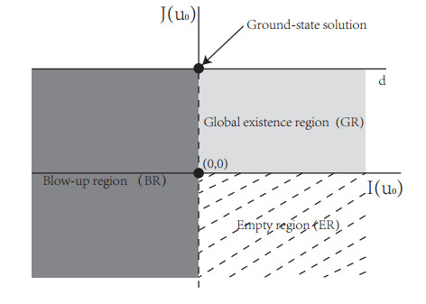
This paper deals with the global existence and blow-up of solutions to a inhomogeneous pseudo-parabolic equation with initial value $ u_0 $ in the Sobolev space $ H_0^1( \Omega) $, where $ \Omega\subset \mathbb{R}^n $ ($ n\geq1 $ is an integer) is a bounded domain. By using the mountain-pass level $ d $ (see (14)), the energy functional $ J $ (see (12)) and Nehari function $ I $ (see (13)), we decompose the space $ H_0^1( \Omega) $ into five parts, and in each part, we show the solutions exist globally or blow up in finite time. Furthermore, we study the decay rates for the global solutions and lifespan (i.e., the upper bound of blow-up time) of the blow-up solutions. Moreover, we give a blow-up result which does not depend on $ d $. By using this theorem, we prove the solution can blow up at arbitrary energy level, i.e. for any $ M\in \mathbb{R} $, there exists $ u_0\in H_0^1( \Omega) $ satisfying $ J(u_0) = M $ such that the corresponding solution blows up in finite time.

| [1] |
Basic concepts in the theory of seepage of homogeneous liquids in fissured rocks. J. Appl. Math. Mech. (1960) 24: 1286-1303. 
|
| [2] |
T. B. Benjamin, J. L. Bona and J. J. Mahony, Model equations for long waves in nonlinear dispersive systems, Philos. Trans. Roy. Soc. London Ser. A, 272 (1972), 47–78. doi: 10.1098/rsta.1972.0032
|
| [3] |
Y. Cao and J. X. Yin, Small perturbation of a semilinear pseudo-parabolic equation, Discrete Contin. Dyn. Syst., 36 (2016), 631–642. doi: 10.3934/dcds.2016.36.631
|
| [4] |
Y. Cao, J. X. Yin and C. P. Wang, Cauchy problems of semilinear pseudo-parabolic equations, J. Differential Equations, 246 (2009), 4568–4590. doi: 10.1016/j.jde.2009.03.021
|
| [5] |
Y. Cao, Z. Y. Wang and J. X. Yin., A semilinear pseudo-parabolic equation with initial data non-rarefied at $\infty$, J. Func. Anal., 277 (2019), 3737–3756. doi: 10.1016/j.jfa.2019.05.014
|
| [6] | T. Cazenave and A. Haraux, An Introduction to Semilinear Evolution Equations, volume 13 of Oxford Lecture Series in Mathematics and its Applications. The Clarendon Press, Oxford University Press, New York, 1998. Translated from the 1990 French original by Yvan Martel and revised by the authors. |
| [7] |
H. F. Di, Y. D. Shang and X. M. Peng, Blow-up phenomena for a pseudo-parabolic equation with variable exponents, Appl. Math. Lett., 64 (2017), 67–73. doi: 10.1016/j.aml.2016.08.013
|
| [8] | H. Fujita, On the blowing up of solutions of the Cauchy problem for $u_{t} = \Delta u+u^{1+\alpha }$, J. Fac. Sci. Univ. Tokyo Sect. I, 13 (1966), 109–124. |
| [9] |
Y. Z. Han, Finite time blowup for a semilinear pseudo-parabolic equation with general nonlinearity, Appl. Math. Lett., 99 (2020), 105986, 7pp. doi: 10.1016/j.aml.2019.07.017
|
| [10] |
S. M. Ji, J. X. Yin and Y. Cao, Instability of positive periodic solutions for semilinear pseudo-parabolic equations with logarithmic nonlinearity, J. Differential Equations, 261 (2016), 5446–5464. doi: 10.1016/j.jde.2016.08.017
|
| [11] |
H. A. Levine, Instability and nonexistence of global solutions of nonlinear wave equation of the form $Pu_tt = Au + F(u)$, Trans. Amer. Math. Soc., 192 (1974), 1–21. doi: 10.2307/1996814
|
| [12] |
Z. P. Li and W. J. Du, Cauchy problems of pseudo-parabolic equations with inhomogeneous terms, Z. Angew. Math. Phys., 66 (2015), 3181–3203. doi: 10.1007/s00033-015-0558-2
|
| [13] |
W. J. Liu and J. Y. Yu, A note on blow-up of solution for a class of semilinear pseudo-parabolic equations, J. Funct. Anal., 274 (2018), 1276–1283. doi: 10.1016/j.jfa.2018.01.005
|
| [14] |
Y. C. Liu and J. S. Zhao, On potential wells and applications to semilinear hyperbolic equations and parabolic equations, Nonlinear Anal., 64 (2006), 2665–2687. doi: 10.1016/j.na.2005.09.011
|
| [15] |
Blow-up phenomena for a pseudo-parabolic equation. Math. Methods Appl. Sci. (2015) 38: 2636-2641.
|
| [16] |
M. Marras, S. V.-Piro and G. Viglialoro, Blow-up phenomena for nonlinear pseudo-parabolic equations with gradient term, Discrete Contin. Dyn. Syst. Ser. B, 22 (2017), 2291–2300. doi: 10.3934/dcdsb.2017096
|
| [17] |
V. Padrón, Effect of aggregation on population recovery modeled by a forward-backward pseudoparabolic equation, Tran. Amer. Math. Soc., 356 (2004), 2739–2756. doi: 10.1090/S0002-9947-03-03340-3
|
| [18] |
L. E. Payne and D. H. Sattinger, Saddle points and instability of nonlinear hyperbolic equations, Israel J. Math., 22 (1975), 273–303. doi: 10.1007/BF02761595
|
| [19] |
D. H. Sattinger, On global solution of nonlinear hyperbolic equations, Arch. Rational Mech. Anal., 30 (1968), 148–172. doi: 10.1007/BF00250942
|
| [20] |
R. E. Showalter and T. W. Ting, Pseudoparabolic partial differential equations, SIAM J. Math. Anal., 1 (1970), 1–26. doi: 10.1137/0501001
|
| [21] |
F. L. Sun, L. S. Liu and Y. H. Wu, Finite time blow-up for a class of parabolic or pseudo-parabolic equations, Comput. Math. Appl., 75 (2018), 3685–3701. doi: 10.1016/j.camwa.2018.02.025
|
| [22] |
R. Temam, Infinite-dimensional Dynamical Systems in Mechanics and Physics, volume 68 of Applied Mathematical Sciences., Springer-Verlag, New York, 1988. doi: 10.1007/978-1-4684-0313-8
|
| [23] |
T. W. Ting, Certain non-steady flows of second-order fluids, Arch. Rational Mech. Anal., 14 (1963), 1–26. doi: 10.1007/BF00250690
|
| [24] | G. Y. Xu and J. Zhou, Lifespan for a semilinear pseudo-parabolic equation, Math. Methods Appl. Sci., 41 (2018), 705–713. |
| [25] |
R. Z. Xu and Y. Niu, Addendum to "Global existence and finite time blow-up for a class of semilinear pseudo-parabolic equations" [J. Func. Anal., 264 (2013) 2732–2763] [ MR3045640], J. Funct. Anal., 270 (2016), 4039–4041. doi: 10.1016/j.jfa.2016.02.026
|
| [26] |
R. Z. Xu and J. Su, Global existence and finite time blow-up for a class of semilinear pseudo-parabolic equations, J. Funct. Anal., 264 (2013), 2732–2763. doi: 10.1016/j.jfa.2013.03.010
|
| [27] |
R. Z. Xu, X. C. Wang and Y. B. Yang, Blowup and blowup time for a class of semilinear pseudo-parabolic equations with high initial energy, Appl. Math. Lett., 83 (2018), 176–181. doi: 10.1016/j.aml.2018.03.033
|
| [28] |
C. X. Yang, Y. Cao and S. N. Zheng, Second critical exponent and life span for pseudo-parabolic equation, J. Differential Equations, 253 (2012), 3286–3303. doi: 10.1016/j.jde.2012.09.001
|
| [29] |
X. L. Zhu, F. Y. Li and Y. H. Li, Some sharp results about the global existence and blowup of solutions to a class of pseudo-parabolic equations, Proc. Roy. Soc. Edinburgh Sect. A, 147 (2017), 1311–1331. doi: 10.1017/S0308210516000494
|

Figures(2)
Jun Zhou. Initial boundary value problem for a inhomogeneous pseudo-parabolic equation[J]. Electronic Research Archive, 2020, 28(1): 67-90. doi: 10.3934/era.2020005


 DownLoad: