An efficiency dynamic seasonal regression forecasting technique for high variation of water level in Yom River Basin of Thailand

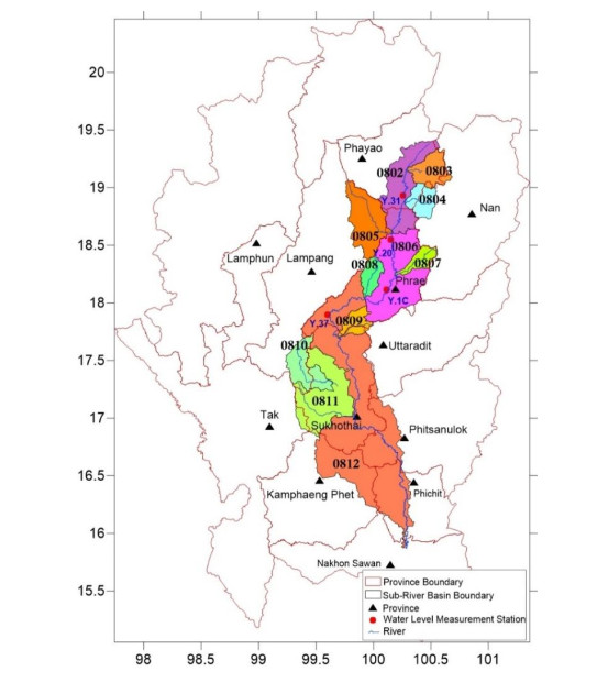
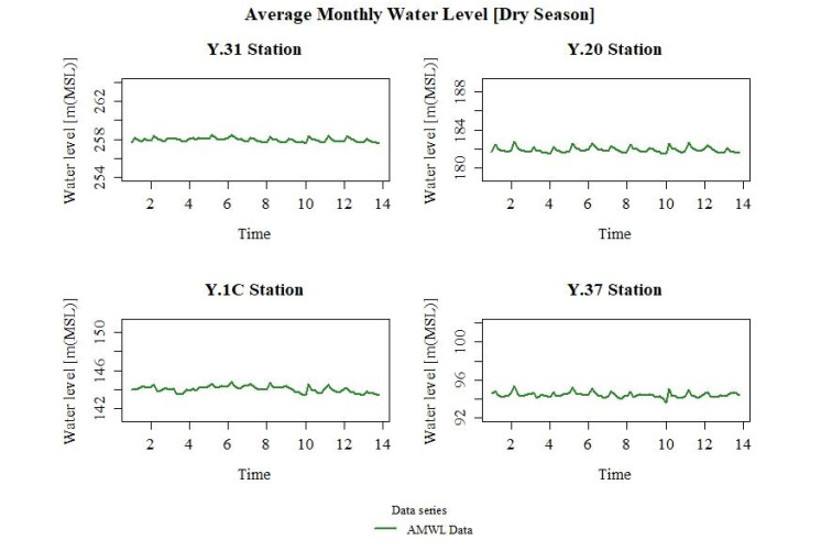
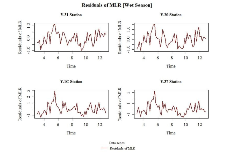
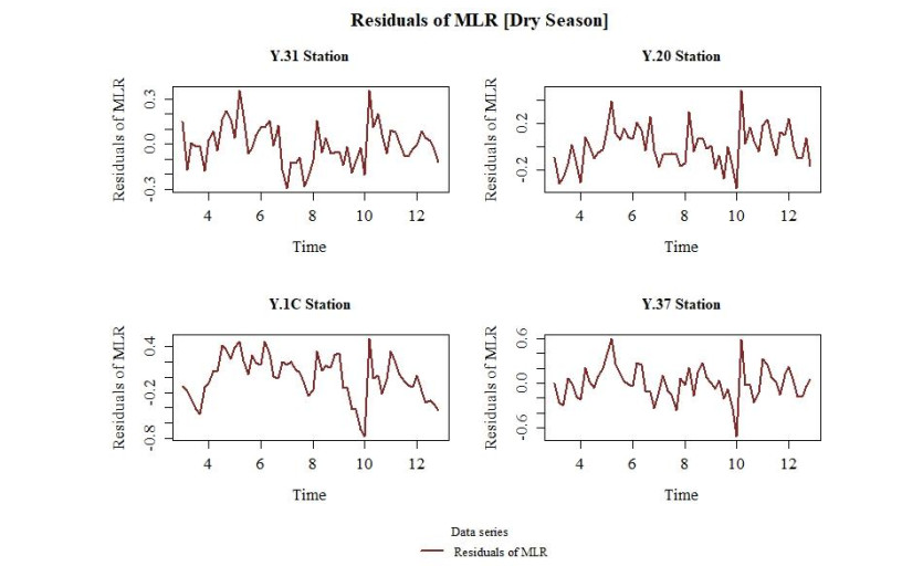
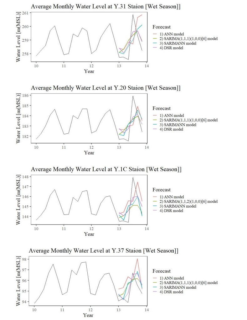
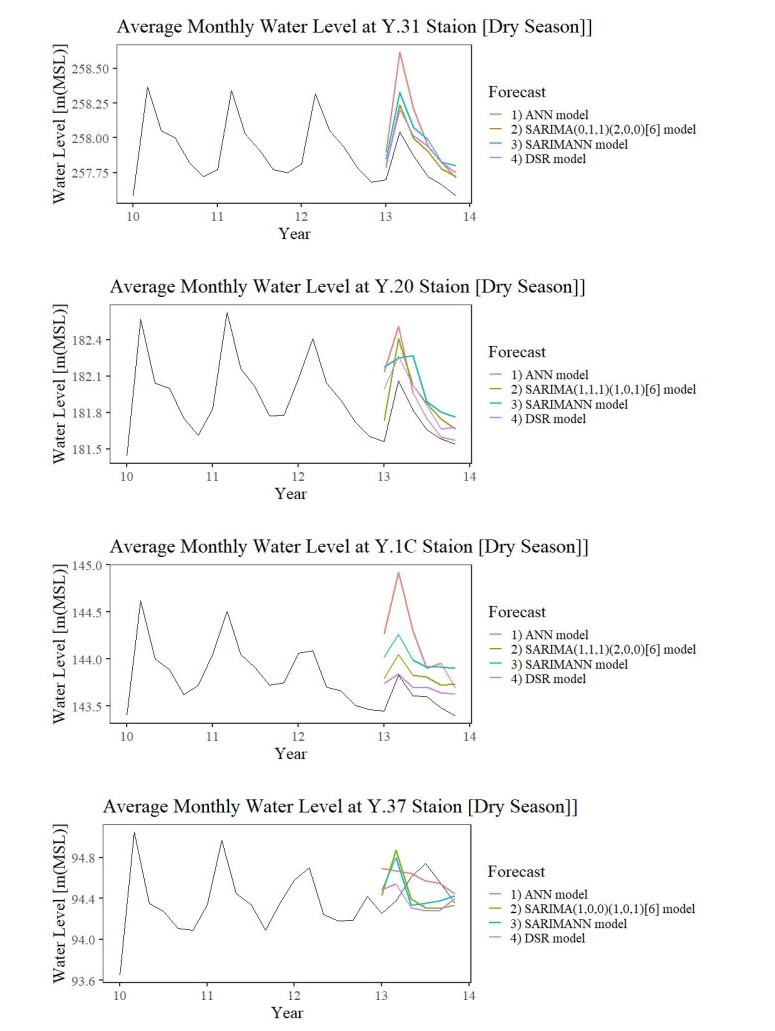
1.   Introduction

In the last 15 years, US deaths due to the opioid epidemic have quadrupled from nearly 12,000 in 2002 to more than 47,000 in 2017 ^[1]. In October 2017, the US Department of Health and Human Services declared the opioid crisis a national public health emergency ^[2]. The increase in injection drug use and reduction of behavioral inhibition have also contributed to the spread of infectious diseases, particularly HIV ^[3]. The two epidemics – opioid and HIV – are intertwined and modeling them in tandem will lead to understanding their interdependence ^[4].

The HIV epidemic, which begun in 1981, has been modeled extensively both on immunological level and on epidemiological level. On within-host level typically models involve healthy and infected CD4 cells and the virus ^[5,6,7,8,9]. On the between-host scale, the very basic models include susceptible, infected and AIDS classes ^[10,11]. Multi-scale models of HIV, mostly of the nested type ^[12], have also received significant attention in the recent years ^{[13,14,15,16]}.

Modeling of the opioid epidemic is more recent and picked up with the increasing importance of the substance abuse disorder. Early models ^[17] assume opioid use can be modeled similarly to infectious disease spread and that assumption has been used in current models of heroin use ^{[18,19,20,21]}. The transition to opioid use typically starts from prescription drug misuse and modeling of that has also been drawing attention lately ^[22].

Despite the importance of the HIV and the opioid epidemics and the clear interdependence between the two, relatively little modeling has been done at the interface of the two epidemics. The within-host modeling of the interplay between opioid and HIV has first drawn attention. Based on experiments in monkeys, Vaidya et al. ^{[23,24,25,26]} model the within-host dynamics of HIV and an opioid. The between host dynamics has been addressed even less. Duan et al. ^[27] models the two epidemics on population level and finds that the best control strategy should reduce the probability of opioid affected individuals getting HIV and should target the drug abuse epidemic. In this paper, we investigate the interplay of the two epidemics with a multi-scale model that incorporates both a within-host component and a between host component.

The sexual contacts leading to HIV are not homogeneous across the population. Typically, few individuals in the population partake in a lot of contacts, while most of the members of the population partake in few contacts. This type of heterogeneity of contacts in HIV transmission is modeled by scale-free networks. Modeling infectious disease dynamics on networks has been also drawing attention in the recent years, resulting in a book devoted to this topic ^[28]. We use here a network modeling approach introduced in ^[29] which gives a closed form model equations ^[30]. In this modeling framework of networks, ODE and age structured models have been investigated but the only multi-scale model on networks in closed form seems to be ^[16]. Here we expand the modeling framework developed in ^[16] to include the opioid epidemic thus considering for the first time a multi-scale network model of two diseases. This model is in closed form and we are able to perform analysis on it.

In Section 2 we introduce the multi-scale network model of HIV and opioid which consists of within-host component, between-host component and linking functions used to connect the two scales. In Section 3 we discuss the existence and stability of the disease-free equilibrium and compute an explicit form of the reproduction numbers. In Section 4 we focus on the existence and stability of the semi-trivial equilibria. In Section 4 we also compute the invasion numbers of the two epidemics. In Section 5 we perform simulations and consider different scenarios with differing parameter values. In Section 6 we summarize our results.

2.   The model

2.1.   The within-host model

We modify a well-known within-host model of HIV by explicitly including the opioid drug concentration $C(\tau)$ and its impact on the average susceptibility of target cells. The model takes the following form.

Here $T$ are the target cells, $T_i$ are the infected target cells and $V_i$ is the virus (HIV). Target cells are produced at rate $s$ and cleared at rate $d_T$. Infected cells die at a rate $\delta_i$, releasing $N_v$ viral particles at death. The clearance rate of the virus is denoted by $c$. Opioid is taken at doses $\Lambda$ is degraded at rate $d_c$. Infection rate of target cells by HIV in the presence of opioid is given by

where $C_0$ is the half saturation constant, $k_0$ is the transmission coefficient in the absence of opioid and $k_1$ is a maximal increase in infection rate due to opioids.

A shortcoming of this model is that it does not consider multiple infection routes and drug resistant viral strains. This problem could have been remedied if a model such as the one formulated in ^[31] was used instead, as the base model. But because of the network structure, the system is already complicated, and addition of strains and infection route would further complicate it. We believe addition of strains and infection route would not give any different insights with the network structures.

2.2.   The between-host model

To introduce the model, we define a complex network with size (number of nodes) $N$ where each node is either occupied by an individual or vacant. The states for the epidemic transmission process on the network are divided into vacant state $E$, susceptible state $S$, opioid state $U$, infected state $V$, co-affected state $i(\tau, t)$ and AIDS state $A$. Nodes change states at rates to be introduced, and HIV transmission is governed by the network connections. A vacant state becomes susceptible state at the recruitment rate. Susceptible, opioid, infected, co-affected and AIDS states can change their state into a vacant state at natural death rate $\mu$ or at disease-induced death rates $d_u$, $d_v$, $d_i(\tau)$, $d_a$, respectively. A susceptible state can be infected with HIV and change into an infected state, or can become opioid-dependent and change into opioid state. HIV and opioid states can get co-affected by adding the other disease. An opioid state or co-affected state can move to a susceptible or HIV-infected states respectively due to treatment denoted as $\delta$. HIV-infected or co-affected states can move to the AIDS state at rates $\gamma_v$ and $\gamma_i(\tau)$.

For an epidemic network, degree of a node is the number of contacts the node has with other nodes. We assume that the network contacts are HIV type contacts. That is an edge between any two nodes represents a potential for transmission of HIV, either through sexual contact or intravenous drug usage. For a network with maximal degree $n$, the average network degree is given by

where $p(k)$ is the probability that a randomly chosen node has degree $k$. That is, $< k >$ is a constant, when $n$ is pre-specified. This is a standard notation for average degree. For further background, ^[32] is a good source for network science. Empirical studies suggest that many real-life HIV networks have scale-free degree distribution $p(k)\sim k^{-\eta}$, where $2 < \eta < 3$ ^[33,34]. The conditional probability $p(j | k)$ that a node with degree $k$ is connected to a node with degree $j$, is given by

Basically, $p(j | k)$ gives probability that an individual with $k$ contacts is connected to an individual with $j$ contacts. We assume contacts that lead to opioid addiction are homogeneous (transmission of opioid addiction can be between two nodes with the same probability). With the structure of a complex network and infection age, let $S_k(t)$, $U_k(t)$, $V_k(t)$, $A_k(t)$, be the number of susceptible, opioid-dependent, HIV infected and AIDS nodes respectively with degree $k$ at time $t$ for $k\in \{1, 2, \dots, n\}$. Let $i_k(\tau, t)$ be the density of co-affected nodes of degree $k$ at time $t$ and with infection age $\tau$. Then we can formulate the following network multi-scale model of HIV and opioid epidemics.

The total population size of degree $k$ is $N_k(t) = S_k(t)+U_k(t)+V_k(t)+I_k(t)$ where $I_k(t) = \int_{0}^{\infty}i_{k}(t, \tau)d\tau$. The force of HIV infection, $\lambda_v(t)$ takes into account the heterogeneous mixing in the network:

Thus $\lambda_v^k(t)$ denotes the force of infection from a node with degree $k$, where $\beta^k_{v_1}$ is the infection rate from $V_k(t)$ (HIV-infected node with degree $k$) per effective contact, and similarly, $\beta^k_{v_2}(\tau)$ is the time-since-infection dependent infection rate from $i_k(\tau, t)$ (co-affected node with degree $k$) per effective contact. Then the force of infection $\lambda_v(t)$ for the heterogeneous network model is obtained by summing over all the degrees of the network $\lambda_v^k(t)$ times the probability that the node with degree $k$ is linked to the node with degree $j$. This is the average force of infection from each contact, and is therefore multiplied by $k$ in the equations (2.2) for HIV transmission to nodes of degree $k$. The force of opioid addiction, $\lambda_u(t)$ is then given by,

Since the opioid contacts are homogeneous within the network, the force of addiction is obtained by summing over all the force of addictions of degree $k$, $\lambda_u^k(t)$. The within-host model remains the same as in (2.1) and the linking functions are given below.

2.3.   Linking functions

To link the within-host and between host models, we use data ^[35] to determine the form of the linking of the transmission coefficient $\beta^{k}_{v_2}(\tau)$ ^[36] to the viral load. Fitting to the data ^[36], we obtain the following function for $\beta^{k}_{v_2}(\tau)$:

where $r\approx 1$. Further, we use the suggested functions in ^[37] to link the remaining $\tau$-dependent rates:

where $\beta_0^k, B, d_0, d_1, \gamma_0, \sigma_0,$ are constants. Disease-induced death rate $d_i$ and transition to AIDS rate $\gamma_i$ do not depend explicitly on the viral load because the viral load is high during the acute HIV phase but these rates are low during this same stage.

3.   Existence and stability of the disease free equilibrium

Equilibria are time-independent solutions of the system and often determine its long-term behavior. We find the equilibria of this system by setting the derivatives with respect to $t$ equal to zero.

At the disease-free equilibrium $U_{k}(t)$, $V_{k}(t)$ and $i_{k}(t, \tau)$ are zero for all $k$. So, the disease-free equilibrium is given by

To determine the stability of the disease free equilibrium and to find the basic reproduction numbers of HIV infection and opioid addiction, denoted by $\mathcal{R}_{u}$ and $\mathcal{R}_{v}$ respectively, we linearize the system around the disease-free equilibrium. We take $S_{k}(t) = S_{k}^{0} + x_{k}(t)$, $U_{k}(t) = u_{k}(t)$, $V_{k}(t) = v_{k}(t)$, $N_{k}(t) = N_{k}^{0}+n_{k}(t)$ and $i_{k}(t, \tau) = y_{k}(t, \tau)$. Then linearizing the system (2.2) takes the following form

where,

We look for solutions of the form $x_{k}(t) = x_{k0}e^{\lambda t}$, $u_{k}(t) = u_{k0}e^{\lambda t}$, $v_{k}(t) = v_{k0}e^{\lambda t}$, $y_{k}(t, \tau) = y_{k}(\tau)e^{\lambda t}$ and obtain the following eigenvalue problem,

Solving the fourth equation of (3.3) we get

where

Substituting (3.4) in the second equation of (3.3) we have,

We notice that all $u_{k0}$ have the same sign. Summing both sides from $1$ to $n$ after dividing with $N_{k}^{0}$, we get

If $\sum_{k = 1}^{n}\frac{u_{k0}}{N_{k}^{0}} = 0$ then $u_{k0} = 0$ for all $k$ which is not the case. So cancelling $\sum_{k = 1}^{n}\frac{u_{k0}}{N_{k}^{0}}$ from both sides of the equation we obtain,

since $N_k^0 = S_k^0 = \frac{\Lambda_k}{\mu}$. We define

Substituting (3.4) in the third equation of (3.3) we have,

We note that all $v_{k0}$ have the same sign. Multiplying both sides by $\frac 1{ < k > }\sum_{k = 1}^n kp(k) \frac{\beta^k_{v_1}}{N_k^{0}}$ and summing from $1$ to $n$ we obtain,

If $\frac{1}{ < k > }\sum_{k = 1}^n kp(k) \frac{\beta^k_{v_1}v_{k0}}{N_k^{0}} = 0$, then $v_{k0} = 0$ for all $k$ which is not the case. So cancelling $\frac 1{ < k > }\sum_{k = 1}^n kp(k) \frac{\beta^k_{v_1}v_{k0}}{N_k^{0}}$ from both sides we get,

So we define

Now we can prove the following theorem,

Theorem 1. If $\max\{\mathcal{R}_{u}, \mathcal{R}_{v}\} < 1$ then the disease free equilibrium is locally asymptotically stable. If $\max\{\mathcal{R}_{u}, \mathcal{R}_{v}\} > 1$, then the disease-free equilibrium is unstable.

Proof. Suppose

Then we notice that $\mathcal{G}_{1}(0) = \mathcal{R}_{u}$, $\mathcal{G}_{2}(0) = \mathcal{R}_{v}$, $\lim_{\lambda \to \infty}\mathcal{G}_{1}(\lambda) = 0$, $\lim_{\lambda \to \infty}\mathcal{G}_{2}(\lambda) = 0$.

We claim that if $\max\{\mathcal{R}_{u}, \mathcal{R}_{v}\} < 1$ then the disease free equilibrium is locally asymptotically stable, that is all the solutions of $\mathcal{G}_{1}(\lambda) = 1$ and $\mathcal{G}_{2}(\lambda) = 1$, have negative real parts. To show this, we proceed by way of contradiction. Suppose one of the equations $\mathcal{G}_{1}(\lambda) = 1$ and $\mathcal{G}_{2}(\lambda) = 1$ has a solution $\lambda_{0}$ with $\Re{(\lambda_{0})} \geq 0$. Then,

or

This is a contradiction. Hence $\varepsilon^{0}$ is locally asymptotically stable when $\max\{\mathcal{R}_{u}, \mathcal{R}_{v}\} < 1$. If $\max\{\mathcal{R}_{u}, \mathcal{R}_{v}\} > 1$, let us assume, without loss of generality, $\mathcal{R}_{u} > 1$. Then $\mathcal{G}_{1}(\lambda) = 1$ has a positive solution, $\lambda^{*}$. Thus, the disease free equilbrium is unstable.

4.   Semi-trivial (Boundary) equilibria

4.1.   Existence of semi-trivial equilibria

In this section, we prove the existence and stability of the two boundary equilibria $E_1^*$ and $E_2^*$ corresponding to opioid addiction and HIV transmission in a single population respectively. To obtain $E_1^*$ we let $S_k(t) = S_{k1}^*$, $U_{k}(t) = U_{k1}^*$ and $V_{k}(t) = 0$ and $i_{k}(t, \tau) = 0$ for all $k$, i.e., $E_1^* = (S_{11}^*, U_{11}^{*}, 0, 0, \cdots, S_{n1}^{*}, U_{n1}^{*}, 0, 0)$. We get the following equations

From the second equation of (4.1) we get,

Summing both sides of the equation from $k = 1$ to $k = n$, and dividing by $N_{k1}^{*}$ we get,

We know $\frac{S_{k1}^{*}+U_{k1}^{*}}{N_{k1}^*} = 1$, and so

i.e.,

Plugging in the values in the first equation of (4.1) and solving for $U_{k1}^{*}$ we get

Now when $\mathcal{R}_{u} < 1$, $\sum_{k = 1}^{n}\frac{U_{k1}^{*}}{N_{k1}^{*}} < 0$, which implies $U_{k1}^{*} < 0$ for at least one $k$. When $\mathcal{R}_{u} > 1$, $U_{k1}^{*} > 0$. Thus, $E_{1}^{*}$ exists if and only if $\mathcal{R}_{u} > 1$.

To obtain $E_2^*$ we let $S_k(t) = S_{k2}^*$, $V_{k}(t) = V_{k2}^*$ and $U_{k}(t) = 0$ and $i_{k}(t, \tau) = 0$ for all $k$, i.e., $E_2^* = (S_{12}^*, 0, V_{12}^{*}, 0, \cdots, S_{n2}^{*}, 0, V_{n2}^{*}, 0)$. We get the following equations

From the second equation of (4.5) we get

Dividing both sides by $N_{k2}^{*}$ and multiplying with $\frac 1{ < k > }\sum_{k = 1}^n kp(k)\beta^k_{v_1}$ and adding from $1$ to $n$ we get,

We know $\frac{S_{k2}^{*}+V_{k2}^{*}}{N_{k2}^*} = 1$, and so

which gives us,

So when $\mathcal{R}_{v} < 1$, $E_{2}^{*}$ does not exist. Now

and so we obtain,

$\lambda_{v}(V_{2}^{*}) = 0$ is a solution to (4.5) which gives the disease free equilibrium. Then for a boundary equilibrium, $\lambda_{v}(V_{2}^{*}) > 0$ is a root of $f(\lambda_{v})$, where

As $\lambda_{v}$ increases $f$ decreases. $\lim_{\lambda_{v} \to \infty} f(\lambda_{v}) = -1$. But $f(0) = \mathcal{R}_{v} -1 > 0$. Then if $\mathcal{R}_{v} > 1$, $f(\lambda_{v})$ has a unique zero, giving us a unique boundary equilibrium for the system.

4.2.   Stability of boundary equilibria and invasion numbers

To find the invasion number of HIV and stability of $E_{1}^{*}$ we first linearize the system (2.2) around $E_{1}^{*}$. We set $S_{k}(t) = x_{k}(t)+S_{k1}^{*}$, $U_{k}(t) = u_{k}(t)+U_{k1}^{*}$, $V_{k}(t) = v_{k}(t)$, $i_{k}(t, \tau) = y_{k}(t, \tau)$ and $N_{k}(t) = n_{k}(t)+N_{k1}^{*}$, the system for the perturbations becomes,

where,

We look for solutions of the form $x_{k}(t) = x_{k}e^{\lambda t}$, $u_{k}(t) = u_{k}e^{\lambda t}$, $v_{k}(t) = v_{k}e^{\lambda t}$, $y_{k}(\tau, t) = y_{k}(\tau)e^{\lambda t}$ and obtain the following eigenvalue problem,

where,

and

Now, using the third, fourth and fifth equation of (4.11) we will compute the invasion number of HIV.

From the second equation of (4.2) we get $y_{k}(\tau) = y_k(0)\pi(\tau)e^{-\frac{\lambda\tau}{k_s}}$, where $\pi(\tau)$ is as defined before. Suppose $K = \beta_{u}q_{u}\sum_{k = 1}^{n}\frac{U_{k1}^{*}}{N_{k1}^{*}}$ and $Q(\lambda) = \delta[\int_0^{\infty} \sigma(\tau)\pi(\tau) e^{-\frac{\lambda\tau}{k_s}} d\tau]$. Then from the first and third equations of (4.2) we get,

Solving for $v_k$ and $y_k(0)$ we obtain,

Supplying these values in Eq (4.12), and cancelling $\lambda_v(v, y)$ from both sides of the equation, we obtain,

We define

We call $\mathcal{R}^{1}_{v_i}$ the invasion reproduction number of HIV infection. Now suppose,

$\int_{0}^{\infty} \beta^{j}_{v_2}(\tau) e^{-\lambda \tau} \pi(\tau) d\tau = \beta_{j}(\lambda)$. $\beta_{j}(\lambda)$ is bounded above by $\beta_{j}(0)$ and $Q(\lambda)$ is bounded above by $Q(0)$. Then $\mathcal{G}_{vi}(0) = \mathcal{R}^{1}_{v_i}$ and $\lim_{\lambda \to \infty} \mathcal{G}_{vi}(\lambda) = 0$. Suppose (4.14) has a solution $\lambda = x+iy$ with $\Re({\lambda}) = x\ge0$ and $\mathcal{R}_{vi}^{1} < 1$. First we prove the following result.

Proof. To prove (4.16) we write down the left hand side of the inequality,

where, $C_1 = \frac{U_{j1}^{*}}{N_{j1}^{*}}$, $C_2 = \frac{S_{j1}^{*}}{N_{j1}^{*}}$ and $z = \sqrt{(x+\mu+d_v+\gamma_v+K)^{2}+y^{2}}$. Since $f'(z) < 0$, $f(z)$ is a decreasing function. That is when $z(0, 0)\leq z(x, y)$, $f(z(0, 0))\geq f(z(x, y))$. But $f(z(0, 0))$ is just the right hand side of (4.16). Using (4.16) we can now state the following,

This is a contradiction. So (4.14) only has solutions with non-negative real parts when $\mathcal{R}_{vi}^{1} < 1$.

Now let us suppose, $\mathcal{R}^{1}_{vi} > 1$. It can be shown that $\mathcal{G}_{vi}(\lambda)$ is decreasing. Then since $\mathcal{G}_{vi}(0) = \mathcal{R}^{1}_{v_i} > 1$ and $\lim_{\lambda \to \infty} \mathcal{G}_{vi}(\lambda) = 0$ for real and positive $\lambda$, (4.14) must have at least one positive root when $\mathcal{R}_{vi} > 1$. Now, from (4.1)–(4.3) we get,

i.e.,

Solving the equation we get,

To find the remaining eigenvalues, satisfying the third, fourth and fifth equation of (4.11), $y_{j}(\tau) = 0$ and $v_j = 0$ for all $j = 1, 2, \cdots, n$. The first two equations then just reduce to

Adding the two equations and solving for $n_{k}$ we get

i.e.,

Replacing $x_{k}$ and $n_{k}$ in the second equation of (4.19) we get,

Multiplying both sides of the equation $\frac{1}{N_{k1}^{*}}$ and summing over $1$ to $n$,

$\sum_{j = 1}^{n}\frac{u_{j}}{N_{j1}^{*}} = 0$ implies from (4.20) all $u_k$ would be zero, which would not be of interest. $\sum_{j = 1}^{n}\frac{u_{j}}{N_{j1}^{*}}\neq 0$ for non-equilibrium points, and cancelling the expression on both sides, then the characteristic equation becomes,

Rewriting this equation as a quadratic equation, we get

Simplifying the equation, we have $\lambda^2 +b \lambda +c = 0$ where $b = \mu+\beta_{u}n > 0$ and $c = \left(1-\frac{1}{\mathcal{R}_{u}}\right)\left(\beta_{u}n(\mu+d_u)-(\mu+d_u+\delta)d_{u}\right) > 0$ since, $\beta_{u}n > (\mu+d_{u}+\delta)$ when $\mathcal{R}_{u} > 1$. Hence this quadratic equation has only roots with negative real parts. Combining the work above we can conclude,

Theorem 2. The unique boundary equilibrium $E_{1}^{*}$ is locally asymptotically stable if $\mathcal{R}^{1}_{v_i} < 1$, and it is unstable if $\mathcal{R}^{1}_{v_i} > 1$.

To find the invasion number of opioid addiction and stability of $E_{2}^{*}$ we first linearize the system (2.2) around $E_{2}^{*}$. We set $S_{k}(t) = x_{k}(t)+S_{k2}^{*}$, $U_{k}(t) = u_{k}(t)$, $V_{k}(t) = v_{k}(t)+V_{k2}^{*}$, $i_{k}(t, \tau) = y_{k}(t, \tau)$ and $N_{k}(t) = n_{k}(t)+N_{k2}^{*}$. The system for the perturbations becomes,

where,

and

We look for solutions of the form $x_{k}(t) = x_{k}e^{\lambda t}$, $u_{k}(t) = u_{k}e^{\lambda t}$, $v_{k}(t) = v_{k}e^{\lambda t}$, $y_{k}(t, \tau) = y_{k}(\tau)e^{\lambda t}$ and obtain the following eigenvalue problem,

From the fourth equation of (4.25) we get

Let $Q(\lambda) = \int_{0}^{\infty}\pi(\tau)e^{\frac{-\lambda}{k_s}\tau}d\tau.$ From the second equation of (4.25) we get

Multiplying both sides of this equation with $\frac{1}{N_{k2}^{*}}$ we get,

From the fifth equation of (4.25) we get,

Multiplying both sides of this equation with $\frac{Q(\lambda)}{N_{k2}^{*}}$ we get,

Summing both side of (4.27) and (4.28) from $1$ to $n$ and adding together we get,

where, $S(\lambda) = \sum_{j = 1}^{n}\frac{u_{j}+y_{j}(0)Q(\lambda)}{N_{j2}^{*}}.$ Since $S(\lambda) = 0$ implies from (4.27) $u_k = 0$ for all $k$, $S(\lambda)\neq0$. We cancel $S(\lambda)$ from both sides and get,

Let $\Pi = \int_{0}^{\infty}\pi(\tau)d\tau$. We define

We call $\mathcal{R}^{2}_{u_i}$ the invasion reproduction number of opioid addiction. We claim that when $\mathcal{R}^{2}_{u_i} < 1$ the boundary equilibrium $E_{2}^{*}$ is locally asymptotically stable, that is all the roots of (4.30) have negative real parts. Suppose

Then $\mathcal{G}_{ui}(0) = \mathcal{R}^{2}_{u_i}$ and $\lim_{\lambda \to \infty}\mathcal{G}_{ui}(\lambda) = 0$. Assume the Eq (4.30) has roots with non-negative real part $\Re (\lambda) > 0$. The Eq (4.30) satisfies,

This is a contradiction. Hence all roots of (4.30) have negative real parts when $\mathcal{R}^{2}_{u_i} < 1$. Now let us suppose, $\mathcal{R}^{2}_{u_i} > 1$. Then since $\mathcal{G}'_{ui}(\lambda) < 0$ when $\lambda > 0$, $\mathcal{G}_{ui}(\lambda)$ is decreasing when $\lambda > 0$. But we have, $\mathcal{G}_{ui}(0) = \mathcal{R}^{2}_{u_i} > 1$ and $\lim_{\lambda \to \infty}\mathcal{G}_{ui}(\lambda) = 0$. Then (4.30) has at least one positive root when $\mathcal{R}^{2}_{u_i} > 1$. If $\lambda$ is not a solution of characteristic equation (4.30), we have $u_j = 0$, $y_j(0) = 0$, the remaining two equations of (4.25) then just reduce to

Adding the two equations and solving for $n_{k}$ we get

i.e.,

Using these values for $n_{k}$ and $x_{k}$ in the second equation of (4.33) we get

Dividing both sides by $N_{k2}^{*}$ and readjusting we obtain,

Multiplying both sides of this equation with $\frac 1{ < k > }\sum_{k = 1}^n kp(k) \beta^k_{v_1}(\lambda+\mu+(d_v+\gamma_v)\frac{V_{k2}^{*}}{N_{k2}^{*}})$, we get,

where $T(\lambda) = \frac 1{ < k > }\sum_{j = 1}^n jp(j) \frac{\beta^j_{v_1}v_{j}}{N_{j2}^{*}} \left(\lambda+\mu+(d_v+\gamma_v)\frac{V_{j2}^{*}}{N_{j2}^{*}}\right)$. Since $T(\lambda) = 0$ implies from (4.35), $v_k = 0$ for all $k$, $T(\lambda) \neq 0$ and we get the following characteristic equation,

From (4.8) we obtain,

Assume the Eq (4.37) has roots with non-negative real part. Using (4.9), $\Re \lambda \ge 0$ the Eq (4.37) satisfies,

This is a contradiction. So we can state the following theorem,

Theorem 3. The unique boundary equilibrium $E_{2}^{*}$ is locally asymptotically stable if $\mathcal{R}^{2}_{u_i} < 1$, and is unstable if $\mathcal{R}^{2}_{u_i} > 1$.

5.   Numerical simulations

5.1.   Numerical scheme and simulation

We present a numerical scheme for the immuno-epidemiological models (2.1) and (2.2). The within-host model, consisting of ordinary differential equations can be solved by a stiff ODE solver in MATLAB.

For the between-host model we introduce a finite-difference method. We discretize the domain

where A is a maximal infection age and time $T < \infty$, a maximal time. We take $\Delta t = \Delta \tau$, with $k_s = 1$, and so the points in age and line direction can be computed as,

Setting $M = \left[\frac{A}{\Delta t}\right]$ and $N = \left[\frac{T}{\Delta t}\right]$, we obtain $A = M\Delta t$, $T = N\Delta t$. The numerical method computes approximations to the solution at the mesh points. We assume $S_k(t_j) = S_k^j$, $U_k(t_j) = U_k^j$, $V_k(t_j) = V_k^j$ and $i_k(t_j, \tau_m) = i^j_{m, k}$. We summarize the numerical method below,

To study the coexistence equilibrium analytically is not feasible for this model. So we take the help of simulations to predict the existence of coexistence equilibrium in a scale free network scenario. We consider specific parameter values for which $\mathcal{R}^{2}_{u_i}$ and $\mathcal{R}^{1}_{v_i}$ are greater than 1. The simulations suggest that the coexistence equilibrium exists and is stable. Given parameter values are constant, the invasion number of HIV, $\mathcal{R}^{1}_{v_i}$, seem to show dependence on the size of the network used. With the same parameter values given in Table 3, when the network contains 200 nodes, $\mathcal{R}^{1}_{v_i}$ is close to $1.4$, while with 300 nodes, $\mathcal{R}^{1}_{v_i}$ increases to $2.9$. The invasion number of opioid addiction $\mathcal{R}^{1}_{v_i}$ remains stable near the same value $1.2$ when size of the network is increased from 200 nodes to 300 nodes. This is to be expected since the spread of opioid has been considered homogeneous over the network. Simulations suggesting a coexistence equilibrium are shown in Figure 1.

5.2.   Effects of the parametric values of $q_u$, $q_v$ and $\delta$

We define U(t) = $\sum_{k = 1}^{n}U_k(t)$ as the total opioid addicted population. Similarly we define $V(t)$, $I(t)$ and $S(t)$ as the total HIV infected, total co-infected and total susceptible population respectively. The network utilized had $200$ nodes. The parameters $\beta_u$ and $\beta^{k}_{v_1}$ are estimated by the following formulas, $\beta_{u} = \mathcal{R}_u(\mu + d_u + \delta);$ and $\beta^{k}_{v1} = \mathcal{R}_{v}(\mu+d_v+\gamma_v)$. Since the model we consider does not include treatment for HIV, we consider $\mathcal{R}_v = 5.5$. This estimate is an average value collected from ^[39], which gives an estimation of basic reproduction number of HIV in Rural South West Uganda. Estimated value of $\mathcal{R}_u$ according to ^[27] would be close to $1.1$. Given the fact that a high percentage of US citizens mentioned it would be easy for someone to access opioids for illicit purposes, according to a poll conducted in 2018 (46 percent) and people who misuse opioids often get them from a family member or friend who has a prescription ^[40], we considered the $\mathcal{R}_u$ to be higher in range, around $3.25$. The maximal degree $n$ for the following simulations (except Figure 1) is $43$, with number of nodes being $200$.

The two parameters in (2.2) that are of particular interest are $q_u$ and $q_v$, which determine how much one epidemics impacts the other. That is $q_v$ determines how likely opioid users are to get infected by HIV compared to non-users, and $q_u$ determines how likely HIV infected people are to become opioid addicted compared to non-infected people. In ^[27] the estimated value of the $q_v$ term equivalent was 94.5, and in ^[38], the estimated value of $q_v$ was 30.62. Both estimates suggest a high dependence effect of opioid usage on HIV infection. In our simulations we take the lesser estimate of $q_v = 30.62$. The total co-affected population due to varying values of $q_v$ is simulated, such as $0.5 q_v, q_v, 1.5q_v, 2q_v, 2.5q_v, 3q_v.$ The estimated value for $q_u$ in ^[38] was below 1, but HIV-infected persons are more likely to have chronic pain, receive opioid analgesic treatment, receive higher doses of opioids, and to have substance use disorders and mental illness compared with the general population, putting them at increased risk for opioid use disorder ^[41]. So the simulations were done with the fitted value for $q_u$ along with double, five times and ten times the fitted value. While the total number of co-affected varies according to the network, the trend seems to be similar, with $q_v$ increasing, the total number of co-affected increases (Figure 2). A definite situation of interest is when $q_u = 4.3$, the maximum value seems to be achieved when $q_v$ is close to $60$, not at the highest value of approximately $90$. The simulation was repeated with these values for different network sizes and provided the same result.

A second set of simulations were performed, taking the base value of $q_u = 1.72$. The four individual cases have all other parameters and network values same, only $q_v$ is varied, from $15, 31, 62$ and $93$ respectively. While some of the cases do have permutations, over all the trend is similar, and opposite to the simulations in Figure 2. That is $q_u$ increasing causes the total number of co-affected to decrease (Figure 3). Again we notice a situation of interest, when $q_v = 60$, the maximum value seems to be achieved when $q_u$ is close to $1.72$, not at the lowest value of approximately $0.86$. Repeated simulation with differing sized networks did not show changes in the results.

Another parameter of interest is $\delta$, which denotes the rate of recovery from addiction in the epidemiological model. The estimate for that in ^[27] is close to $0.033$, while in ^[38] the estimate is approximately $0.11$. If successful treatment is considered without subtracting the relapses, the rate would probably be close to $0.05$ ^[42]. To simulate for differing values of $\delta$, we consider $\beta_u$ and $\beta^{k}_{v1}$ as constants, directly taking the values from Table 3. All the other parameter values are as mentioned in Table 3. We consider four differing situations for $\delta$, with the value being $0.02$, the fitted value $0.11$, and target high values of $0.5$ and $\delta = 1$. We also investigated different scenarios with differing network sizes, with number of nodes being $100$, $300$ and $500$ respectively. Interestingly, irrespective of network size, the total number of co-affected people appeared to be higher with the value of $\delta$ increasing (Figure 4). One quite plausible explanation would be the higher recovery would decrease the number of opioid overdose deaths significantly, thereby increasing the co-affected prevalence.

6.   Discussion

We formulate a within-host model linked with a dynamic network HIV/opioid coinfection epidemiological model with demography, through epidemiological parameters. The system is described by ordinary differential equations coupled with partial differential equations in a nested fashion. The network multi-scale model here is an extension of the multi-scale model considered in ^[38]. The disease free equilibrium of the system always exists and is locally asymptotically stable when both the basic reproduction numbers of opioid and HIV, $\mathcal{R}_u$ and $\mathcal{R}_v$ are less than 1.

The boundary equilibrium $E_{1}^*$ exists when $\mathcal{R}_u$ is more than 1 and $E_{2}^*$ exist when $\mathcal{R}_v$ is more than 1. We define the invasion reproduction numbers $\mathcal{R}^{1}_{v_i}$ and $\mathcal{R}^{2}_{u_i}$. The invasion reproduction number $\mathcal{R}^{2}_{u_i}$ gives the reproduction of the opioid users when the population is at the equilibrium $E_2^{*}$, that is, when HIV infection alone is at equilibrium in the single population. The invasion reproduction number $\mathcal{R}^{1}_{v_i}$ gives the reproduction of the HIV infection at the equilibrium $E_1^{*}$, that is when the opioid transmission alone is at equilibrium in the single population. When $\mathcal{R}^{1}_{v_i} < 1$, $E_{1}^*$ is locally stable and when $\mathcal{R}^{1}_{v_i} > 1$, $E_{1}^*$ is unstable. When $\mathcal{R}^{2}_{u_i} < 1$, $E_{2}^*$ is locally stable and when $\mathcal{R}^{2}_{u_i} > 1$, $E_{2}^*$ is unstable. The model is too complicated to compute or consider the stability of an endemic equilibrium, analytically, but simulations suggest that there is an interior equilibrium potentially under the condition that both invasion numbers are larger than one.

We use fitted parameters from ^[38], to perform simulations, to explore the effect of the change of the parameters $q_u$, $q_v$ and $\delta$. The parameters $q_u$ and $q_v$ represent the effect of one epidemic on the other, and we simulated for plausible values of $q_u$ and $q_v$, to get estimates of co-affected prevalence. The estimate of $q_v$, the likelihood of a heroin user to be infected with HIV, in ^[27] was approximately 94, and since a large number of opioid users progress to becoming heroin users, (Data from 2011 showed that an estimated 4 to 6 percent who misuse prescription opioids switch to heroin and about 80 percent of people who used heroin first misused prescription opioids) ^[43], chances of the $q_v$ estimate for all illicit opioid usage being close to the "heroin only" estimate is high. We notice that increase in $q_v$ causes the co-affected population to rise significantly, which indicates that control strategies focusing on reducing HIV infection among the opioid addicted population would be effective in decoupling the epidemics, corroborating with the conclusions in ^[27].

To the best of our knowledge, there have not been previous models with a parameter similar to $q_u$, that provides an estimate for the effect of HIV infection on opioid use. The simulations from our model show that increase of $q_u$ in general causes the number of co-affected to decline. That is the prevalence of co-affected people declines sharply with the increase to more HIV infected people being addicted to opioids. This does corroborate real life data, since deaths due to overdose in the US per year were aproximately 120,000 in the year 2020, and the number increased 15 percent by 2021 ^[44], compared to the number of deaths due to HIV being around 18,500 in 2020 ^[45]. We noticed significant increase in the prevalence of co-affected individuals, when the parameter $\delta$, representing the recovery from opioid usage was increased significantly. The sharp increase points to the idea that control measures should focus more on treatment of opioid use disorder, and that uncoupling the two epidemics is a priority to prevent loss of human lives. Counseling about the dangers of opioid addiction for HIV infected people must be provided, and similarly counseling about the dangers of getting infected with HIV should be provided to reported opioid addicts.

In summary, we have developed a novel multi-scale network model of HIV and opioid epidemics. We have analized the model and obtained conditions for HIV-only to persist or opioid-only to persist. Simulations suggest that the two epidemics can co-exist for some parameter values. Simulations further suggest that decreasing $q_v$ decreases the number of co-affected and may lead to decopuling the epidemics. Thus control measures targeted at reducing $q_v$ should be coupled with treatment of opioid affected individuals which is consistent with our previois findings.

Acknowledgments

Maia Martcheva was partially supported by NSF DMS-1951595. Necibe Tuncer was partially supported by NSF DMS-1951626.

Conflict of interest

The authors declare there is no conflict of interest.

Code availability

The code was written by one of the authors and is available on request by contacting Churni Gupta.