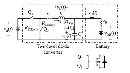
A comprehensive analysis of a two-level battery charger model is presented, focusing on its switched and averaged dynamics validated via MATLAB Simulink simulations. The system, powered by an 800 V DC source, is managed by a robust PI-compensated feedback loop, delivering minimal ripple, rapid transient response, and high stability under varying load conditions. Results demonstrate precise battery current control with a 4 ms settling time for step changes and ripple levels kept below 0.16% for current and 2.4% for capacitor voltage. Sensitivity analyses highlight the impact of non-ideal resistances—such as MOSFET on-resistance and inductor resistance—on efficiency and equilibrium voltage stability. Stability and loop gain studies confirm robust control performance, with all poles positioned in the stable region of the s-plane, ensuring reliable operation. This work provides key insights for designing high-efficiency, stable battery chargers and supports the use of advanced control techniques to further enhance converter performance.
Citation: José M. Campos-Salazar, Juan L. Aguayo-Lazcano, Roya Rafiezadeh. Non-ideal two-level battery charger—modeling and simulation[J]. AIMS Electronics and Electrical Engineering, 2025, 9(1): 60-80. doi: 10.3934/electreng.2025004
A comprehensive analysis of a two-level battery charger model is presented, focusing on its switched and averaged dynamics validated via MATLAB Simulink simulations. The system, powered by an 800 V DC source, is managed by a robust PI-compensated feedback loop, delivering minimal ripple, rapid transient response, and high stability under varying load conditions. Results demonstrate precise battery current control with a 4 ms settling time for step changes and ripple levels kept below 0.16% for current and 2.4% for capacitor voltage. Sensitivity analyses highlight the impact of non-ideal resistances—such as MOSFET on-resistance and inductor resistance—on efficiency and equilibrium voltage stability. Stability and loop gain studies confirm robust control performance, with all poles positioned in the stable region of the s-plane, ensuring reliable operation. This work provides key insights for designing high-efficiency, stable battery chargers and supports the use of advanced control techniques to further enhance converter performance.

| [1] |
Khaligh A, D'Antonio M (2019) Global Trends in High-Power On-Board Chargers for Electric Vehicles. IEEE T Veh Technol 68: 3306–3324. https://doi.org/10.1109/TVT.2019.2897050 doi: 10.1109/TVT.2019.2897050

|
| [2] |
Tu H, Feng H, Srdic S, Lukic S (2019) Extreme Fast Charging of Electric Vehicles: A Technology Overview. IEEE T Transp Electr 5: 861–878. https://doi.org/10.1109/TTE.2019.2958709 doi: 10.1109/TTE.2019.2958709
|
| [3] |
Rahimi-Eichi H, Ojha U, Baronti F, Chow MY (2013) Battery Management System: An Overview of Its Application in the Smart Grid and Electric Vehicles. IEEE Ind Electron Mag 7: 4–16. https://doi.org/10.1109/MIE.2013.2250351 doi: 10.1109/MIE.2013.2250351
|
| [4] |
Sfakianakis GE, Everts J, Lomonova EA (2015) Overview of the Requirements and Implementations of Bidirectional Isolated AC-DC Converters for Automotive Battery Charging Applications. Proceedings of the 2015 Tenth International Conference on Ecological Vehicles and Renewable Energies (EVER), 1–12. https://doi.org/10.1109/EVER.2015.7112939 doi: 10.1109/EVER.2015.7112939
|
| [5] |
Kim JM, Lee J, Eom TH, Bae KH, Shin MH, Won CY (2018) Design and Control Method of 25kW High Efficient EV Fast Charger. Proceedings of the 2018 21st International Conference on Electrical Machines and Systems (ICEMS), 2603–2607. https://doi.org/10.23919/ICEMS.2018.8549491 doi: 10.23919/ICEMS.2018.8549491
|
| [6] |
Ronanki D, Kelkar A, Williamson SS (2019) Extreme Fast Charging Technology—Prospects to Enhance Sustainable Electric Transportation. Energies 12: 3721. https://doi.org/10.3390/en12193721 doi: 10.3390/en12193721
|
| [7] | Medén A (2023) DC-DC Converter for Fast Charging with Mobile BESS in a Weak Grid 2023. |
| [8] |
Kilicoglu H, Tricoli P (2023) Technical Review and Survey of Future Trends of Power Converters for Fast-Charging Stations of Electric Vehicles. Energies 16: 5204. https://doi.org/10.3390/en16135204 doi: 10.3390/en16135204
|
| [9] |
Ketsingsoi S, Kumsuwan Y (2014) An Off-Line Battery Charger Based on Buck-Boost Power Factor Correction Converter for Plug-in Electric Vehicles. Energy Procedia 56: 659–666. https://doi.org/10.1016/j.egypro.2014.07.205 doi: 10.1016/j.egypro.2014.07.205
|
| [10] |
Tofoli FL, Pereira D, de C Josias de Paula W, Oliveira Júnior D de S (2015) Survey on Non-Isolated High-Voltage Step-up Dc–Dc Topologies Based on the Boost Converter. IET Power Electron 8: 2044–2057. https://doi.org/10.1049/iet-pel.2014.0605 doi: 10.1049/iet-pel.2014.0605
|
| [11] |
Rim C, Joung GB, Cho GH (1988) A State-Space Modeling of Nonideal DC-DC Converters. PESC 88 Record 19th Annual IEEE Power Electronics Specialists Conference (1988), 943–950. https://doi.org/10.1109/PESC.1988.18229 doi: 10.1109/PESC.1988.18229
|
| [12] |
Molina-Santana E, Gonzalez-Montañez F, Liceaga-Castro JU, Jimenez-Mondragon VM, Siller-Alcala I (2023) Modeling and Control of a DC-DC Buck–Boost Converter with Non-Linear Power Inductor Operating in Saturation Region Considering Electrical Losses. Mathematics 11: 4617. https://doi.org/10.3390/math11224617 doi: 10.3390/math11224617
|
| [13] |
Siddhartha V, Hote YV (2018) Systematic Circuit Design and Analysis of a Non-Ideal DC–DC Pulse Width Modulation Boost Converter. IET Circ Device Syst 12: 144–156. https://doi.org/10.3390/math11224617 doi: 10.3390/math11224617
|
| [14] |
Iqbal M, Benmouna A, Becherif M, Mekhilef S (2023) Survey on Battery Technologies and Modeling Methods for Electric Vehicles. Batteries 9: 185. https://doi.org/10.3390/batteries9030185 doi: 10.3390/batteries9030185
|
| [15] | Erickson RW, Maksimovic D (2013) Fundamentals of Power Electronics, Springer Science & Business Media. |
| [16] | Mohan N (1995) Power Electronics: Converters, Applications, and Design, Wiley. |
| [17] | Alepuz S (2004) Aportación al control del convertidor CC/CA de tres niveles, Universitat Politècnica de Catalunya. |
| [18] | Katsuhiko O (2009) Modern Control Engineering, Boston. |
| [19] |
Thingvad A, Ziras C, Marinelli M (2019) Economic Value of Electric Vehicle Reserve Provision in the Nordic Countries under Driving Requirements and Charger Losses. J Energy Storage 21: 826–834. https://doi.org/10.1016/j.est.2018.12.018 doi: 10.1016/j.est.2018.12.018
|
| [20] |
Lee J, Kim JM, Yi J, Won CY (2021) Battery Management System Algorithm for Energy Storage Systems Considering Battery Efficiency. Electronics 10: 1859. https://doi.org/10.3390/electronics10151859 doi: 10.3390/electronics10151859
|
| [21] |
Su X, Sun B, Wang J, Ruan H, Zhang W, Bao Y (2023) Experimental Study on Charging Energy Efficiency of Lithium-Ion Battery under Different Charging Stress. J Energy Storage 68: 107793. https://doi.org/10.1016/j.est.2023.107793 doi: 10.1016/j.est.2023.107793
|
| [22] | Khalil H (2014) Nonlinear Control, 1st edition, Pearson: Boston. |
| [23] | Husain I (2010) Electric and Hybrid Vehicles: Design Fundamentals, 2nd edition, CRC Press. |


Figures(15) / Tables(3)

José M. Campos-Salazar, Juan L. Aguayo-Lazcano, Roya Rafiezadeh. Non-ideal two-level battery charger—modeling and simulation[J]. AIMS Electronics and Electrical Engineering, 2025, 9(1): 60-80. doi: 10.3934/electreng.2025004


 DownLoad: