VV-hemorphin-5 association to lipid bilayers and alterations of membrane bending rigidity

Iva Valkova; Petar Todorov; Victoria Vitkova; Iva Valkova; Petar Todorov; Victoria Vitkova

doi:10.3934/biophy.2022025

AIMS Biophysics

2022, Volume 9, Issue 4: 294-307. doi: 10.3934/biophy.2022025

Previous Article Next Article

Research article Special Issues

VV-hemorphin-5 association to lipid bilayers and alterations of membrane bending rigidity

1.
Faculty of Pharmacy, Medical University, 2, Dunav str., 1000 Sofia
2.
Drug Design and Development Lab, Sofia Tech Park, 111, Tsarigradsko shose blvd., 1784 Sofia, Bulgaria
3.
Department of Organic Chemistry, University of Chemical Technology and Metallurgy, 8, Kliment Ohridski blvd., 1756 Sofia, Bulgaria
4.
Institute of Solid State Physics, Bulgarian Academy of Sciences, 72, Tsarigradsko Shose blvd., 1784 Sofia, Bulgaria

Received: 31 August 2022 Revised: 04 October 2022 Accepted: 12 October 2022 Published: 25 October 2022

The morphinomimetic properties of hemorphins are intensively studied with regard to new peptide drug developments. In this respect, the investigation of mechanical properties and stability of lipid membranes provides a useful background for advancement in pharmacological applications of liposomes. Here we probed the effect of the endogenous heptapeptide VV-hemorphin-5 (valorphin) on the bending elasticity of biomimetic lipid membranes of 1-palmitoyl-2-oleoyl-sn-glycero-3-phosphocholine (POPC) by analysis of thermal shape fluctuations of nearly spherical giant unilamellar vesicles. In a wide concentration range covering valorphin concentrations applied in nociceptive screening in vivo, we report alterations of the bilayer bending rigidity in a concentration-dependent non-monotonic manner. We performed quantitative characterization of VV-hemorphin-5 association to POPC membranes by isothermal titration calorimetry in order to shed light on the partitioning of the amphiphilic hemorphin between the aqueous solution and membranes. The calorimetric results correlate with flicker spectroscopy findings and support the hypothesis about the strength of valorphin-membrane interaction related to the peptide bulk concentration. A higher strength of valorphin interaction with the bilayer corresponds to a more pronounced effect of the peptide on the membrane's mechanical properties. The presented study features the comprehensive analysis of membrane bending elasticity as a biomarker for physicochemical effects of peptides on lipid bilayers. The reported data on thermodynamic parameters of valorphin interactions with phosphatidylcholine bilayers and alterations of their mechanical properties is expected to be useful for applications of lipid membrane systems in pharmacology and biomedicine.
- valorphin,
- lipid bilayer,
- isothermal titration calorimetry,
- bending elasticity,
- giant unilamellar vesicles,
- thermal fluctuation analysis
Citation: Iva Valkova, Petar Todorov, Victoria Vitkova. VV-hemorphin-5 association to lipid bilayers and alterations of membrane bending rigidity[J]. AIMS Biophysics, 2022, 9(4): 294-307. doi: 10.3934/biophy.2022025

Related Papers:

Abstract

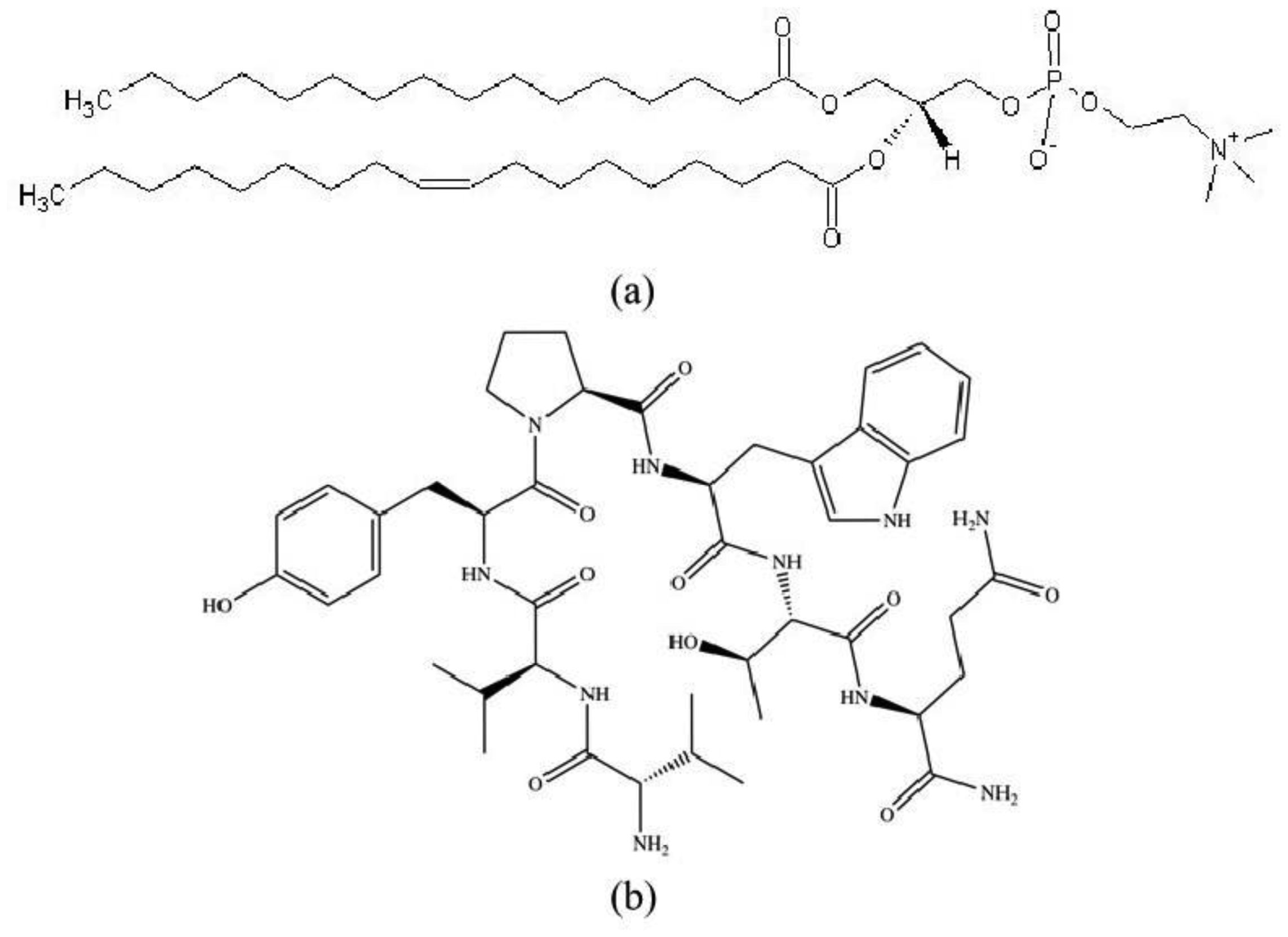
The morphinomimetic properties of hemorphins are intensively studied with regard to new peptide drug developments. In this respect, the investigation of mechanical properties and stability of lipid membranes provides a useful background for advancement in pharmacological applications of liposomes. Here we probed the effect of the endogenous heptapeptide VV-hemorphin-5 (valorphin) on the bending elasticity of biomimetic lipid membranes of 1-palmitoyl-2-oleoyl-sn-glycero-3-phosphocholine (POPC) by analysis of thermal shape fluctuations of nearly spherical giant unilamellar vesicles. In a wide concentration range covering valorphin concentrations applied in nociceptive screening in vivo, we report alterations of the bilayer bending rigidity in a concentration-dependent non-monotonic manner. We performed quantitative characterization of VV-hemorphin-5 association to POPC membranes by isothermal titration calorimetry in order to shed light on the partitioning of the amphiphilic hemorphin between the aqueous solution and membranes. The calorimetric results correlate with flicker spectroscopy findings and support the hypothesis about the strength of valorphin-membrane interaction related to the peptide bulk concentration. A higher strength of valorphin interaction with the bilayer corresponds to a more pronounced effect of the peptide on the membrane's mechanical properties. The presented study features the comprehensive analysis of membrane bending elasticity as a biomarker for physicochemical effects of peptides on lipid bilayers. The reported data on thermodynamic parameters of valorphin interactions with phosphatidylcholine bilayers and alterations of their mechanical properties is expected to be useful for applications of lipid membrane systems in pharmacology and biomedicine.

Acknowledgments

Funding from the National Science Fund of Bulgaria (KP-06-N58/6/2021) is acknowledged.

Conflict of interest

The authors declare no conflict of interest.

Author contributions

Iva Valkova: Visualization, Investigation, Writing—original draft preparation. Petar Todorov: Conceptualization, Resources, Writing—review & editing. Victoria Vitkova: Conceptualization, Methodology, Investigation, Visualization, Writing—original draft preparation.

References

[1]	Karelin AA, Philippova MM, Karelina EV, et al. (1994) Isolation of endogenous hemorphin-related hemoglobin fragments from bovine brain. Biochem Bioph Res Co 202: 410-415. https://doi.org/10.1006/bbrc.1994.1943
[2]	Sanderson K, Nyberg F, Khalil Z (1998) Modulation of peripheral inflammation by locally administered hemorphin-7. Inflamm Res 47: 49-55. https://doi.org/10.1007/s000110050266
[3]	Altinoz MA, Elmaci I, Ince B, et al. (2016) Hemoglobins, hemorphins, and 11p15.5 chromosomal region in cancer biology and immunity with special emphasis for brain tumors. J Neurol Surg Part A 77: 247-257. https://doi.org/10.1055/s-0035-1566120
[4]	Altinoz MA, Guloksuz S, Schmidt-Kastner R, et al. (2019) Involvement of hemoglobins in the pathophysiology of Alzheimer's disease. Exp Gerontol 126: 110680. https://doi.org/10.1016/j.exger.2019.110680
[5]	Blishchenko EY, Sazonova OV, Kalinina OA, et al. (2005) Antitumor effect of valorphin in vitro and in vivo: combined action with cytostatic drugs. Cancer Biol Ther 4: 125-131. https://doi.org/10.4161/cbt.4.1.1474
[6]	Blishchenko EY, Sazonova OV, Kalinina OA, et al. (2002) Family of hemorphins: co-relations between amino acid sequences and effects in cell cultures. Peptides 23: 903-910. https://doi.org/10.1016/S0196-9781(02)00017-7
[7]	Wei F, Zhao L, Jing Y (2020) Hemoglobin-derived peptides and mood regulation. Peptides 127: 170268. https://doi.org/10.1016/j.peptides.2020.170268
[8]	Ali A, Alzeyoudi SAR, Almutawa SA, et al. (2020) Molecular basis of the therapeutic properties of hemorphins. Pharmacol Res 158: 104855. https://doi.org/10.1016/j.phrs.2020.104855
[9]	Mielczarek P, Hartman K, Drabik A, et al. (2021) Hemorphins—From discovery to functions and pharmacology. Molecules 26: 3879. https://doi.org/10.3390/molecules26133879
[10]	Wieprecht T, Seelig J (2002) Isothermal titration calorimetry for studying interactions between peptides and lipid membranes. Curr Top Membr 52: 31-56. https://doi.org/10.1016/S1063-5823(02)52004-4
[11]	Wiseman T, Williston S, Brandts JF, et al. (1989) Rapid measurement of binding constants and heats of binding using a new titration calorimeter. Anal Biochem 179: 131-137. https://doi.org/10.1016/0003-2697(89)90213-3
[12]	Velázquez-Campoy A, Ohtaka H, Nezami A, et al. (2004) Isothermal titration calorimetry. Curr Protoc Cell Biol : 17.18.1-17.18.24. https://doi.org/10.1002/0471143030.cb1708s23
[13]	Todorov P, Peneva P, Pechlivanova D, et al. (2018) Synthesis, characterization and nociceptive screening of new VV-hemorphin-5 analogues. Bioorg Med Chem Lett 28: 3073-3079. https://doi.org/10.1016/j.bmcl.2018.07.040
[14]	Vitkova V, Yordanova V, Staneva G, et al. (2021) Dielectric properties of phosphatidylcholine membranes and the effect of sugars. Membranes-Basel 11: 847. https://doi.org/10.3390/membranes11110847
[15]	Angelova MI, Dimitrov DS (1986) Liposome electroformation. Faraday Discuss Chem Soc 81: 303-311. https://doi.org/10.1039/DC9868100303
[16]	Vitkova V, Antonova K, Popkirov G, et al. (2010) Electrical resistivity of the liquid phase of vesicular suspensions prepared by different methods. J Phys Conf Ser 253: 012059. https://doi.org/10.1088/1742-6596/253/1/012059
[17]	Genova J, Vitkova V, Bivas I (2013) Registration and analysis of the shape fluctuations of nearly spherical lipid vesicles. Phys Rev E 88: 022707. https://doi.org/10.1103/PhysRevE.88.022707
[18]	Mitov MD, Faucon JF, Méléard P, et al. (1992) Thermal fluctuations of membranes, In: Gokel, G.W., Advances in Supramolecular Chemistry, 1 Eds., Greenwich: JAI Press Inc., 93–139.
[19]	Faucon JF, Mitov MD, Méléard P, et al. (1989) Bending elasticity and thermal fluctuations of lipid membranes. Theoretical and experimental requirements. J Phys 50: 2389-2414. https://doi.org/10.1051/jphys:0198900500170238900
[20]	Bivas I, Hanusse P, Bothorel P, et al. (1987) An application of the optical microscopy to the determination of the curvature elastic modulus of biological and model membranes. J Phys 48: 855-867. https://doi.org/10.1051/jphys:01987004805085500
[21]	Schneider MB, Jenkins JT, Webb WW (1984) Thermal fluctuations of large quasi-spherical bimolecular phospholipid vesicles. J Phys 45: 1457-1472. https://doi.org/10.1051/jphys:019840045090145700
[22]	Helfrich W (1973) Elastic properties of lipid bilayers: theory and possible experiments. Z Naturforsch C 28: 693-703. https://doi.org/10.1515/znc-1973-11-1209
[23]	Genova J, Vitkova V, Aladgem L, et al. (2005) Stroboscopic illumination gives new opportunities and improves the precision of bending elastic modulus measurements. J Optoelectron Adv M 7: 257-260.
[24]	Seelig J (1997) Titration calorimetry of lipid–peptide interactions. BBA-Biomembranes 1331: 103-116. https://doi.org/10.1016/S0304-4157(97)00002-6
[25]	Freyer MW, Lewis EA (2008) Isothermal titration calorimetry: experimental design, data analysis, and probing macromolecule/ligand binding and kinetic interactions. Method Cell Biol 84: 79-113. https://doi.org/10.1016/s0091-679x(07)84004-0
[26]	Damian L (2013) Isothermal titration calorimetry for studying protein-ligand interactions, In: Williams, M., Daviter, T., Protein-Ligand Interactions, Methods in Molecular Biology, New Jersey: Humana Press, 1008, 103–118. https://doi.org/10.1007/978-1-62703-398-5_4
[27]	Turner DC, Straume M, Kasimova MR, et al. (1995) Thermodynamics of interaction of the fusion-inhibiting peptide Z-D-Phe-L-Phe-Gly with dioleoylphosphatidylcholine vesicles: direct calorimetric determination. Biochemistry-US 34: 9517-9525. https://doi.org/10.1021/bi00029a028
[28]	Seelig J (2004) Thermodynamics of lipid–peptide interactions. BBA-Biomembranes 1666: 40-50. https://doi.org/10.1016/j.bbamem.2004.08.004
[29]	Tamm LK (1994) Physical studies of peptide—bilayer interactions, In: White, S.H., Membrane Protein Structure, Methods in Physiology Series, New York: Springer, New York. https://doi.org/10.1007/978-1-4614-7515-6_13
[30]	Ben-Shaul A, Ben-Tal N, Honig B (1996) Statistical thermodynamic analysis of peptide and protein insertion into lipid membranes. Biophys J 71: 130-137. https://doi.org/10.1016/S0006-3495(96)79208-1
[31]	Mertins O, Dimova R (2011) Binding of chitosan to phospholipid vesicles studied with isothermal titration calorimetry. Langmuir 27: 5506-5515. https://doi.org/10.1021/la200553t
[32]	Milner ST, Safran SA (1987) Dynamical fluctuations of droplet microemulsions and vesicles. Phys Rev A 36: 4371-4379. https://doi.org/10.1103/PhysRevA.36.4371
[33]	Bivas I (2010) Shape fluctuations of nearly spherical lipid vesicles and emulsion droplets. Phys Rev E 81: 061911. https://doi.org/10.1103/PhysRevE.81.061911
[34]	Fernandez-Puente L, Bivas I, Mitov MD, et al. (1994) Temperature and chain length effects on bending elasticity of phosphatidylcholine bilayers. Europhysics Lett 28: 181-186. https://doi.org/10.1209/0295-5075/28/3/005
[35]	Rawicz W, Olbrich KC, Mclntosh T, et al. (2000) Effect of chain length and unsaturation on elasticity of lipid bilayers. Biophys J 79: 328-339. https://doi.org/10.1016/S0006-3495(00)76295-3
[36]	Marsh D (2006) Elastic curvature constants of lipid monolayers and bilayers. Chem Phys Lipids 144: 146-159. https://doi.org/10.1016/j.chemphyslip.2006.08.004
[37]	Vitkova V, Petrov AG (2013) Lipid bilayers and membranes: material properties, In: Aleš, I., Genova, J., Advances in Planar Lipid Bilayers and Liposomes, Academic Press, 17, 89–138. https://doi.org/10.1016/B978-0-12-411516-3.00005-X
[38]	Dimova R (2014) Recent developments in the field of bending rigidity measurements on membranes. Adv Colloid Interfac 208: 225-234. https://doi.org/10.1016/j.cis.2014.03.003
[39]	Faizi HA, Tsui A, Dimova R, et al. (2022) Bending rigidity, capacitance, and shear viscosity of giant vesicle membranes prepared by spontaneous swelling, electroformation, gel-assisted, and phase transfer methods: a comparative study. Langmuir 38: 10548-10557. https://doi.org/10.1021/acs.langmuir.2c01402
[40]	Dimova R (2019) Giant vesicles and their use in assays for assessing membrane phase state, curvature, mechanics, and electrical properties. Annu Rev Biophys 48: 93-119. https://doi.org/10.1146/annurev-biophys-052118-115342
[41]	Bivas I, Méléard P (2003) Bending elasticity of a lipid bilayer containing an additive. Phys Rev E 67: 012901. https://doi.org/10.1103/PhysRevE.67.012901
[42]	Vitkova V, Méléard P, Pott T, et al. (2006) Alamethicin influence on the membrane bending elasticity. Eur Biophys J 35: 281-286. https://doi.org/10.1007/s00249-005-0019-5
[43]	Shchelokovskyy P, Tristram-Nagle S, Dimova R (2011) Effect of the HIV-1 fusion peptide on the mechanical properties and leaflet coupling of lipid bilayers. New J Phys 13: 025004. https://doi.org/10.1088/1367-2630/13/2/025004
[44]	Bouvrais H, Méléard P, Pott T, et al. (2008) Softening of POPC membranes by magainin. Biophys Chem 137: 7-12. https://doi.org/10.1016/j.bpc.2008.06.004
[45]	Pott T, Gerbeaud C, Barbier N, et al. (2015) Melittin modifies bending elasticity in an unexpected way. Chem Phys Lipids 185: 99-108. https://doi.org/10.1016/j.chemphyslip.2014.05.004
[46]	Zemel A, Ben-Shaul A, May S (2008) Modulation of the spontaneous curvature and bending rigidity of lipid membranes by interfacially adsorbed amphipathic peptides. J Phys Chem B 112: 6988-6996. https://doi.org/10.1021/jp711107y
[47]	Evans E, Rawicz W (1997) Elasticity of “Fuzzy” Biomembranes. Phys Rev Lett 79: 2379-2382. https://doi.org/10.1103/PhysRevLett.79.2379
[48]	Méléard P, Gerbeaud C, Pott T, et al. (1997) Bending elasticities of model membranes: influences of temperature and sterol content. Biophys J 72: 2616-2629. https://doi.org/10.1016/S0006-3495(97)78905-7
[49]	Gracià RS, Bezlyepkina N, Knorr RL, et al. (2010) Effect of cholesterol on the rigidity of saturated and unsaturated membranes: fluctuation and electrodeformation analysis of giant vesicles. Soft Matter 6: 1472-1482. https://doi.org/10.1039/b920629a
[50]	Sugár IP, Bonanno AP, Chong PLG (2018) Gramicidin lateral distribution in phospholipid membranes: fluorescence phasor plots and statistical mechanical model. Int J Mol Sci 19: 3690. https://doi.org/10.3390/ijms19113690
[51]	Wieprecht T, Beyermann M, Seelig J (2002) Thermodynamics of the coil-ɑ-helix transition of amphipathic peptides in a membrane environment: the role of vesicle curvature. Biophys Chem 96: 191-201. https://doi.org/10.1016/s0301-4622(02)00025-x

Reader Comments

Your name:*

Email:*
© 2022 the Author(s), licensee AIMS Press. This is an open access article distributed under the terms of the Creative Commons Attribution License (http://creativecommons.org/licenses/by/4.0)