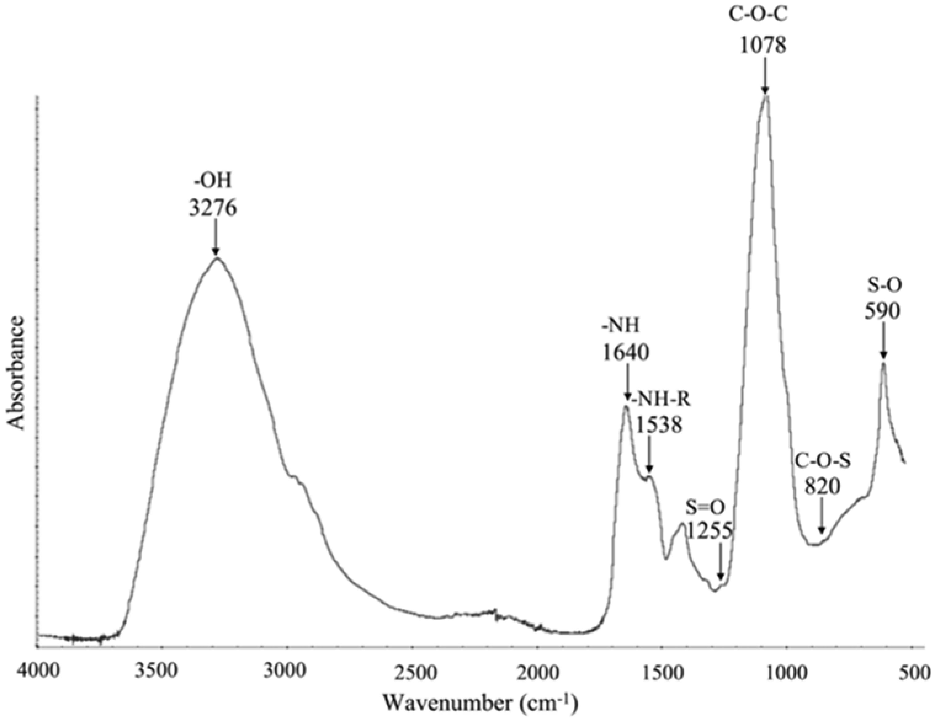
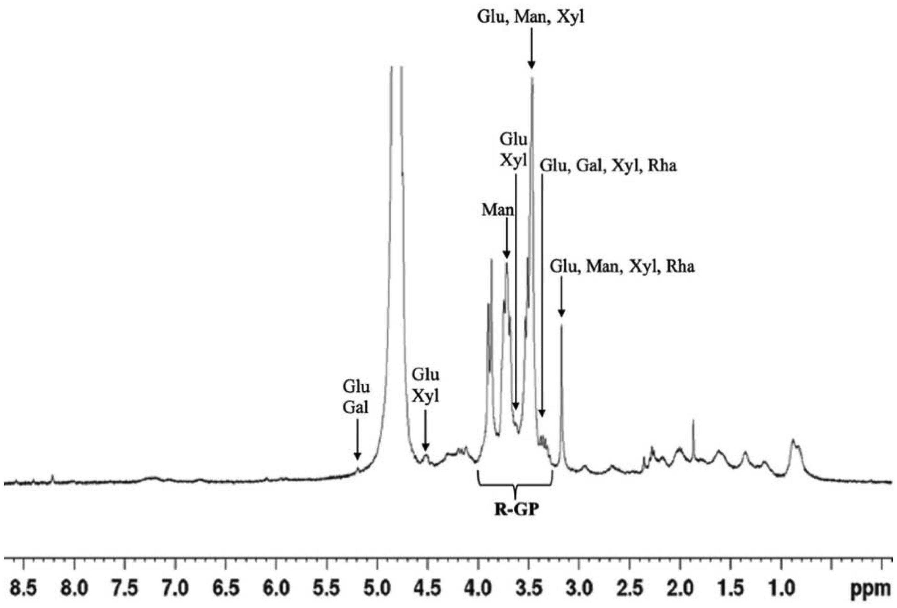
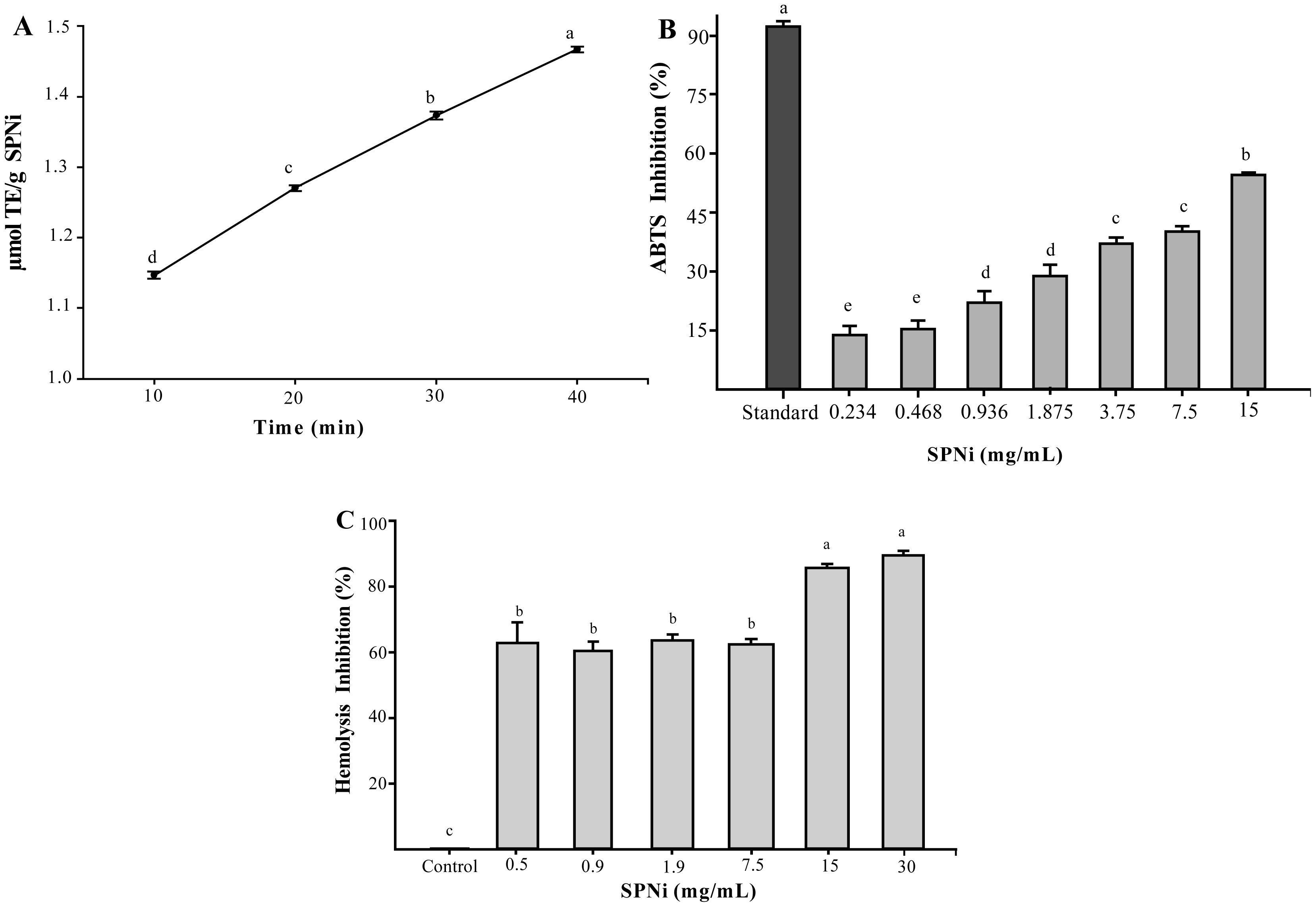
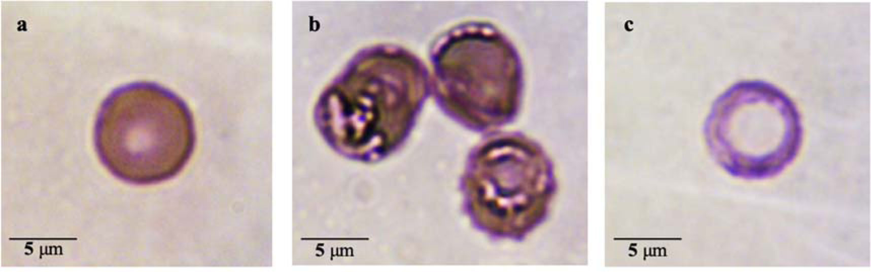
A sulfated polysaccharide from Navicula incerta (SPNi) was extracted, and its physicochemical characteristics, antioxidant activity, and anti-hemolytic property were investigated. The polysaccharide yield was 4.8% (SPNi weight/biomass dry weight). Glucose, galactose, mannose, and xylose were the primary sugars. The sulfate content and Mw values were 0.46% and 45 kDa, respectively. The FT-IR spectrum showed characteristic bands at 3276,1079,1255, and 820 cm−1, related to -OH, C-O-C, S=O, and C-O-S stretching vibration. The 1H-NMR analysis revealed signals of anomeric protons, indicating the presence of CH2-O and CH-O groups. SPNi registered ferric-reducing antioxidant power (up to 1.47 µmol TE/g) and 54% anti-radical activity on ABTS+. This polysaccharide registered 90% hemolysis inhibition achieving integrity of the erythrocyte membrane. The results indicate that SPNi could be a candidate for biotechnology applications where antioxidant activity and hemolysis inhibition are required.
Citation: Ricardo I. González-Vega, Carmen L. Del-Toro-Sánchez, Ramón A. Moreno-Corral, José A. López-Elías, Aline Reyes-Díaz, Norma García-Lagunas, Elizabeth Carvajal-Millán, Diana Fimbres-Olivarría. Sulfated polysaccharide-rich extract from Navicula incerta: physicochemical characteristics, antioxidant activity, and anti-hemolytic property[J]. AIMS Bioengineering, 2022, 9(4): 364-382. doi: 10.3934/bioeng.2022027
A sulfated polysaccharide from Navicula incerta (SPNi) was extracted, and its physicochemical characteristics, antioxidant activity, and anti-hemolytic property were investigated. The polysaccharide yield was 4.8% (SPNi weight/biomass dry weight). Glucose, galactose, mannose, and xylose were the primary sugars. The sulfate content and Mw values were 0.46% and 45 kDa, respectively. The FT-IR spectrum showed characteristic bands at 3276,1079,1255, and 820 cm−1, related to -OH, C-O-C, S=O, and C-O-S stretching vibration. The 1H-NMR analysis revealed signals of anomeric protons, indicating the presence of CH2-O and CH-O groups. SPNi registered ferric-reducing antioxidant power (up to 1.47 µmol TE/g) and 54% anti-radical activity on ABTS+. This polysaccharide registered 90% hemolysis inhibition achieving integrity of the erythrocyte membrane. The results indicate that SPNi could be a candidate for biotechnology applications where antioxidant activity and hemolysis inhibition are required.

| [1] |
Raposo MF de J, de Morais RMSC, de Morais AMM (2013) Bioactivity and applications of sulphated polysaccharides from marine microalgae. Mar Drugs 11: 233-252. https://doi.org/10.3390/md11010233 
|
| [2] |
Staats N, De Winder B, Stal LJ, et al. (1999) Isolation and characterization of extracellular polysaccharides from the epipelic diatoms Cylindrotheca closterium and Navicula salinarum. Eur J Phycol 34: 161-169. https://doi.org/10.1080/09670269910001736212
|
| [3] |
Yim JH, Kim SJ, Ahn SH, et al. (2007) Characterization of a novel bioflocculant, p-KG03, from a marine dinoflagellate, Gyrodinium impudicum KG03. Bioresour Technol 98: 361-367. https://doi.org/10.1016/j.biortech.2005.12.021
|
| [4] | Nomoto K, Yokokura T, Satoh HMM (1983) Antitumor activity of chlorella extract, PCM-4, by oral administration. Cancer Chemother 10: 781-785. |
| [5] |
Yim JH, Kim SJ, Ahn SH, et al. (2004) Antiviral effects of sulfated exopolysaccharide from the marine microalga Gyrodinium impudicum strain KG03. Mar Biotechnol 6: 17-25. https://doi.org/10.1007/s10126-003-0002-z
|
| [6] |
Yu Y, Zhu S, Hou Y, et al. (2020) Sulfur contents in sulfonated hyaluronic acid direct the cardiovascular cells fate. ACS Appl Mater Interfaces 12: 46827-46836. https://doi.org/10.1021/acsami.0c15729
|
| [7] |
Feriani A, Tir M, Hamed M, et al. (2020) Multidirectional insights on polysaccharides from Schinus terebinthifolius and Schinus molle fruits: Physicochemical and functional profiles, in vitro antioxidant, anti-genotoxicity, antidiabetic, and antihemolytic capacities, and in vivo anti-inflammatory and anti-nociceptive properties. Int J Biol Macromol 165: 2576-2587. https://doi.org/10.1016/j.ijbiomac.2020.10.123
|
| [8] |
Meng Q, Chen F, Xiao T, et al. (2019) Inhibitory effects of polysaccharide from Diaphragma juglandis fructus on α-amylase and α-D-glucosidase activity, streptozotocin-induced hyperglycemia model, advanced glycation end-products formation, and H2O2-induced oxidative damage. Int J Biol Macromol 124: 1080-1089. https://doi.org/10.1016/j.ijbiomac.2018.12.011
|
| [9] |
Duan S, Zhao M, Wu B, et al. (2020) Preparation, characteristics, and antioxidant activities of carboxymethylated polysaccharides from blackcurrant fruits. Int J Biol Macromol 155: 1114-1122. https://doi.org/10.1016/j.ijbiomac.2019.11.078
|
| [10] | Yu Y, Zhu SJ, Dong HT, et al. A novel MgF2/PDA/S-HA coating on the bio-degradable ZE21B alloy for better multi-functions on cardiovascular application (2021). https://doi.org/10.1016/j.jma.2021.06.015 |
| [11] |
Wijesinghe WAJP, Jeon YJ (2012) Biological activities and potential industrial applications of fucose rich sulfated polysaccharides and fucoidans isolated from brown seaweeds: A review. Carbohydr Polym 88: 13-20. https://doi.org/10.1016/j.carbpol.2011.12.029
|
| [12] |
Lo TCT, Chang CA, Chiu KH, et al. (2011) Correlation evaluation of antioxidant properties on the monosaccharide components and glycosyl linkages of polysaccharide with different measuring methods. Carbohydr Polym 86: 320-327. https://doi.org/10.1016/j.carbpol.2011.04.056
|
| [13] |
Guerra-Dore CMP, Faustino Alves MG, Pofírio Will LSE, et al. (2013) A sulfated polysaccharide, fucans, isolated from brown algae Sargassum vulgare with anticoagulant, antithrombotic, antioxidant and anti-inflammatory effects. Carbohydr Polym 91: 467-475. https://doi.org/10.1016/j.carbpol.2012.07.075
|
| [14] |
Guillard RRL, Ryther JH (1962) Studies of marine planktonic diatoms: I. Cyclotella Nana Hustedt, and Detonula Confervacea (CLEVE) Gran. Can J Microbiol 8: 229-239. https://doi.org/10.1139/m62-029
|
| [15] |
Fimbres-Olivarria D, Lopez-Elias JA, Carvajal-Millan E, et al. (2016) Navicula sp. Sulfated polysaccharide gels induced by Fe(III): Rheology and microstructure. Int J Mol Sci 17: 1238. https://doi.org/10.3390/ijms17081238
|
| [16] |
Terho TT, Hartiala K (1971) Method for determination of the sulfate content of glycosaminoglycans. Anal Biochem 41: 471-476. https://doi.org/10.1016/0003-2697(71)90167-9
|
| [17] | AOACOfficial Methods of Analysis of AOAC International, Washington DC, USA, Arlington, VA (1995). Available from: http://lib3.dss.go.th/fulltext/scan_ebook/aoac_1995_v78_n3.pdf. |
| [18] |
Rouau X, Surget A (1994) A rapid semi-automated method for the determination of total and water-extractable pentosans in wheat flours. Carbohydr Polym 24: 123-132. https://doi.org/10.1016/0144-8617(94)90022-1
|
| [19] |
Fimbres-Olivarria D, Carvajal-Millan E, Lopez-Elias JA, et al. (2018) Chemical characterization and antioxidant activity of sulfated polysaccharides from Navicula sp. Food Hydrocoll 75: 229-236. https://doi.org/10.1016/j.foodhyd.2017.08.002
|
| [20] |
Lee SY, Mediani A, Maulidiani M, et al. (2018) Comparison of partial least squares and random forests for evaluating relationship between phenolics and bioactivities of Neptunia oleracea. J Sci Food Agric 98: 240-252. https://doi.org/10.1002/jsfa.8462
|
| [21] |
Re R, Pellegrini N, Proteggenete A, et al. (1999) Antioxidant activity applying an improved ABTS radical cation decolorization assay. Free Radic Biol Med 26: 1231-1237. https://doi.org/10.1016/S0891-5849(98)00315-3
|
| [22] |
Benzie I, Strain J (1996) The ferric reducing ability of plasma (FRAP) as a measure of “antioxidant power”: The FRAP assay. Anal Biochem 239: 70-76. https://doi.org/10.1006/abio.1996.0292
|
| [23] |
López-Mata MA, Ruiz-Cruz S, Silva-Beltrán NP, et al. (2013) Physicochemical, antimicrobial and antioxidant properties of chitosan films incorporated with carvacrol. Molecules 18: 13735-13753. https://doi.org/10.3390/molecules181113735
|
| [24] | Lynch EC (1990) Peripheral blood smear. Clinical Methods: The History, Physical, and Laboratory Examinations . Boston: Butterworth 732-734. |
| [25] |
D'Archivio AA, Maggi MA, Ruggieri F (2018) Extraction of curcuminoids by using ethyl lactate and its optimisation by response surface methodology. J Pharm Biomed Anal 149: 89-95. https://doi.org/10.1016/j.jpba.2017.10.042
|
| [26] |
Wiercigroch E, Szafraniec E, Czamara K, et al. (2017) Raman and infrared spectroscopy of carbohydrates: A review. Spectrochim Acta - Part A Mol Biomol Spectrosc 185: 317-335. https://doi.org/10.1016/j.saa.2017.05.045
|
| [27] |
Wang L, Wang X, Wu H, et al. (2014) Overview on biological activities and molecular characteristics of sulfated polysaccharides from marine green algae in recent years. Mar Drugs 12: 4984-5020. https://doi.org/10.3390/md12094984
|
| [28] |
Matsuhiro B (1996) Vibrational spectroscopy of seaweed galactans. Hydrobiologia 326: 481-489. https://doi.org/10.1007/BF00047849
|
| [29] |
Barboríková J, Šutovská M, Kazimierová I, et al. (2019) Extracellular polysaccharide produced by Chlorella vulgaris – Chemical characterization and anti-asthmatic profile. Int J Biol Macromol 135: 1-11. https://doi.org/10.1016/j.ijbiomac.2019.05.104
|
| [30] |
Goo BG, Baek G, Jin Choi D, et al. (2013) Characterization of a renewable extracellular polysaccharide from defatted microalgae Dunaliella tertiolecta. Bioresour Technol 129: 343-350. https://doi.org/10.1016/j.biortech.2012.11.077
|
| [31] |
Huang SQ, Li JW, Li YQ, et al. (2011) Purification and structural characterization of a new water-soluble neutral polysaccharide GLP-F1-1 from Ganoderma lucidum. Int J Biol Macromol 48: 165-169. https://doi.org/10.1016/j.ijbiomac.2010.10.015
|
| [32] |
Rani RP, Anandharaj M, Ravindran A (2018) Characterization of a novel exopolysaccharide produced by Lactobacillus gasseri FR4 and demonstration of its in vitro biological properties. Int J Biol Macromol 109: 772-783. https://doi.org/10.1016/j.ijbiomac.2017.11.062
|
| [33] |
Rajasekar P, Palanisamy S, Anjali R, et al. (2019) Isolation and structural characterization of sulfated polysaccharide from Spirulina platensis and its bioactive potential: In vitro antioxidant, antibacterial activity and Zebrafish growth and reproductive performance. Int J Biol Macromol 141: 809-821. https://doi.org/10.1016/j.ijbiomac.2019.09.024
|
| [34] |
Yuan F, Gao Z, Liu W, et al. (2019) Characterization, antioxidant, anti-aging and organ protective effects of sulfated polysaccharides from flammulina velutipes. Molecules 24: 3517. https://doi.org/10.3390/molecules24193517
|
| [35] |
Trabelsi I, Ben Slima S, Ktari N, et al. (2021) Structure analysis and antioxidant activity of a novel polysaccharide from katan seeds. Biomed Res Int 2021: 6349019. https://doi.org/10.1155/2021/6349019
|
| [36] |
Gurgel Rodrigues JA, Neto ÉM, dos Santos GRC, et al. (2014) Structural analysis of a sulfated polysaccharidic fraction obtained from the coenocytic green seaweed Caulerpa cupressoides var. lycopodium. Acta Sci Technol 36: 203-210. https://doi.org/10.4025/actascitechnol.v36i2.17866
|
| [37] |
Alencar POC, Lima GC, Barros FCN, et al. (2019) A novel antioxidant sulfated polysaccharide from the algae Gracilaria caudata: In vitro and in vivo activities. Food Hydrocoll 90: 28-34. https://doi.org/10.1016/j.foodhyd.2018.12.007
|
| [38] |
Wijesekara I, Pangestuti R, Kim SK (2011) Biological activities and potential health benefits of sulfated polysaccharides derived from marine algae. Carbohydr Polym 84: 14-21. https://doi.org/10.1016/j.carbpol.2010.10.062
|
| [39] |
Moore BG, Tischer RG (1964) Extracellular polysaccharides of algae: effects on life-support systems. Science 145: 586-587. https://doi.org/10.1126/science.145.3632.586
|
| [40] |
Raveendran S, Yoshida Y, Maekawa T, et al. (2013) Pharmaceutically versatile sulfated polysaccharide based bionano platforms. Nanomed Nanotechnol Biol Med 9: 605-626. https://doi.org/10.1016/j.nano.2012.12.006
|
| [41] |
Markou G, Nerantzis E (2013) Microalgae for high-value compounds and biofuels production: A review with focus on cultivation under stress conditions. Biotechnol Adv 31: 1532-1542. https://doi.org/10.1016/j.biotechadv.2013.07.011
|
| [42] |
Han PP, Sun Y, Jia SR, et al. (2014) Effects of light wavelengths on extracellular and capsular polysaccharide production by Nostoc flagelliforme. Carbohydr Polym 105: 145-151. https://doi.org/10.1016/j.carbpol.2014.01.061
|
| [43] |
Borowitzka MA, Beardall J, Raven JA The physiology of microalgae (2016). https://doi.org/10.1007/978-3-319-24945-2
|
| [44] |
Lee JB, Hayashi K, Hirata M, et al. (2006) Antiviral sulfated polysaccharide from Navicula directa, a diatom collected from deep-sea water in toyama bay. Biol Pharm Bull 29: 2135-2139. https://doi.org/10.1248/bpb.29.2135
|
| [45] |
Khandeparker RD, Bhosle NB (2001) Extracellular polymeric substances of the marine fouling diatom amphora rostrata Wm.Sm. Biofouling 17: 117-127. https://doi.org/10.1080/08927010109378471
|
| [46] |
Sudharsan S, Subhapradha N, Seedevi P, et al. (2015) Antioxidant and anticoagulant activity of sulfated polysaccharide from Gracilaria debilis (Forsskal). Int J Biol Macromol 81: 1031-1038. https://doi.org/10.1016/j.ijbiomac.2015.09.046
|
| [47] |
Seedevi P, Moovendhan M, Viramani S, et al. (2017) Bioactive potential and structural chracterization of sulfated polysaccharide from seaweed (Gracilaria corticata). Carbohydr Polym 155: 516-524. https://doi.org/10.1016/j.carbpol.2016.09.011
|
| [48] |
Leandro SM, Gil MC, Delgadillo I (2003) Partial characterisation of exopolysaccharides exudated by planktonic diatoms maintained in batch cultures. Acta Oecologica 24: 49-55. https://doi.org/10.1016/S1146-609X(03)00004-3
|
| [49] |
López-Mata MA, Ruiz-Cruz S, Silva-Beltrán NP, et al. (2015) Physicochemical and antioxidant properties of chitosan films incorporated with cinnamon Oil. Int J Polym Sci 2015: 974506. https://doi.org/10.1155/2015/974506
|
| [50] |
Majdoub H, Mansour M Ben, Chaubet F, et al. (2009) Anticoagulant activity of a sulfated polysaccharide from the green alga Arthrospira platensis. Biochim Biophys Acta Gen Subj 1790: 1377-1381. https://doi.org/10.1016/j.bbagen.2009.07.013
|
| [51] |
Zhang Z, Wang F, Wang X, et al. (2010) Extraction of the polysaccharides from five algae and their potential antioxidant activity in vitro. Carbohydr Polym 82: 118-121. https://doi.org/10.1016/j.carbpol.2010.04.031
|
| [52] |
Fedorov SN, Ermakova SP, Zvyagintseva TN, et al. (2013) Anticancer and cancer preventive properties of marine polysaccharides: Some results and prospects. Mar Drugs 11: 4876-4901. https://doi.org/10.3390/md11124876
|
| [53] |
Ale MT, Mikkelsen JD, Meyer AS (2011) Important determinants for fucoidan bioactivity: A critical review of structure-function relations and extraction methods for fucose-containing sulfated polysaccharides from brown seaweeds. Mar Drugs 9: 2106-2130. https://doi.org/10.3390/md9102106
|
| [54] |
Usov AI (2011) Chapter 4 - Polysaccharides of the red algae. Advances in Carbohydrate Chemistry and Biochemistry . UK: Academic Press 115-217. https://doi.org/10.1016/B978-0-12-385520-6.00004-2
|
| [55] |
Guo JH, Skinner GW, Harcum WW, et al. (1998) Pharmaceutical applications of naturally occurring water-soluble polymers. Pharm Sci Technol Today 1: 254-261. https://doi.org/10.1016/S1461-5347(98)00072-8
|
| [56] |
Melo MRS, Feitosa JPA, Freitas ALP, et al. (2002) Isolation and characterization of soluble sulfated polysaccharide from the red seaweed Gracilaria cornea. Carbohydr Polym 49: 491-498. https://doi.org/10.1016/S0144-8617(02)00006-1
|
| [57] |
Rengasamy KR, Mahomoodally MF, Aumeeruddy MZ, et al. (2020) Bioactive compounds in seaweeds: An overview of their biological properties and safety. Food Chem Toxicol 135: 111013. https://doi.org/10.1016/j.fct.2019.111013
|
| [58] |
Barros FCN, Da Silva DC, Sombra VG, et al. (2013) Structural characterization of polysaccharide obtained from red seaweed Gracilaria caudata (J Agardh). Carbohydr Polym 92: 598-603. https://doi.org/10.1016/j.carbpol.2012.09.009
|
| [59] |
Ale MT, Maruyama H, Tamauchi H, et al. (2011) Fucose-containing sulfated polysaccharides from brown seaweeds inhibit proliferation of melanoma cells and induce apoptosis by activation of caspase-3 in vitro. Mar Drugs 9: 2605-2621. https://doi.org/10.3390/md9122605
|
| [60] |
Patel S (2012) Therapeutic importance of sulfated polysaccharides from seaweeds: updating the recent findings. 3 Biotech 2: 171-185. https://doi.org/10.1007/s13205-012-0061-9
|
| [61] |
Chen C, Zhao Z, Ma S, et al. (2019) Optimization of ultrasonic-assisted extraction, refinement and characterization of water-soluble polysaccharide from Dictyosphaerium sp. and evaluation of antioxidant activity in vitro. J Food Meas Charact 14: 963-977. https://doi.org/10.1007/s11694-019-00346-7
|
| [62] |
Kan Y, Chen T, Wu Y, et al. (2015) Antioxidant activity of polysaccharide extracted from Ganoderma lucidum using response surface methodology. Int J Biol Macromol 72: 151-157. https://doi.org/10.1016/j.ijbiomac.2014.07.056
|
| [63] |
Gómez-Ordóñez E, Jiménez-Escrig A, Rupérez P (2014) Bioactivity of sulfated polysaccharides from the edible red seaweed Mastocarpus stellatus. Bioact Carbohydrates Diet Fibre 3: 29-40. https://doi.org/10.1016/j.bcdf.2014.01.002
|
| [64] | Yarnpakdee S, Benjakul S, Senphan T (2019) Antioxidant activity of the extracts from freshwater macroalgae (Cladophora glomerata) grown in Northern Thailand and its preventive effect against lipid oxidation of refrigerated eastern little tuna slice. Turkish J Fish Aquat Sci 19: 209-219. https://doi.org/10.4194/1303-2712-v19_03_04 |
| [65] | Wang J, Hu S, Nie S, et al. (2016) Reviews on mechanisms of in vitro antioxidant activity of polysaccharides. Oxid Med Cell Longev 2016: 5692852. https://doi.org/10.1155/2016/5692852 |
| [66] |
de Oliveira FC, Coimbra JS dos R, de Oliveira EB, et al. (2016) Food Protein-polysaccharide Conjugates Obtained via the Maillard Reaction: A Review. Crit Rev Food Sci Nutr 56: 1108-1125. https://doi.org/10.1080/10408398.2012.755669
|
| [67] |
Alisi IO, Uzairu A, Abechi SE (2020) Free radical scavenging mechanism of 1,3,4-oxadiazole derivatives: thermodynamics of O–H and N–H bond cleavage. Heliyon 6: e03683. https://doi.org/10.1016/j.heliyon.2020.e03683
|
| [68] | El Kady EM (2019) New Trends of the Polysaccharides as a Drug. World J Agric Soil Sci 3: 1-22. https://doi.org/10.33552/wjass.2019.03.000572 |
| [69] |
Li H, Mao W, Zhang X, et al. (2011) Structural characterization of an anticoagulant-active sulfated polysaccharide isolated from green alga Monostroma latissimum. Carbohydr Polym 85: 394-400. https://doi.org/10.1016/j.carbpol.2011.02.042
|
| [70] |
Guru SMM, Vasanthi M, Achary A (2015) Antioxidant and free radical scavenging potential of crude sulphated polysaccharides from Turbinaria ornata. Biologia (Bratisl) 70: 27-33. https://doi.org/10.1515/biolog-2015-0004
|
| [71] |
Shao P, Chen X, Sun P (2014) Chemical characterization, antioxidant and antitumor activity of sulfated polysaccharide from Sargassum horneri. Carbohydr Polym 105: 260-269. https://doi.org/10.1016/j.carbpol.2014.01.073
|
| [72] | Cao M, Wang S, Gao Y, et al. (2020) Study on physicochemical properties and antioxidant activity of polysaccharides from Desmodesmus armatus. J Food Biochem 44: 1-13. https://doi.org/10.1111/jfbc.13243 |
| [73] |
Díaz-Gutierrez D, Méndez Ortega W, de Oliveira e Silva AM, et al. (2015) Comparation of antioxidants properties and polyphenols content of aqueous extract from seaweeds Bryothamnion triquetrum and Halimeda opuntia. Ars Pharm 56: 89-99. https://doi.org/10.4321/S2340-98942015000200003
|
| [74] | Khalili M, Ebrahimzadeh MA, Safdari Y (2014) Antihaemolytic activity of thirty herbal extracts in mouse red blood cells. Arch Ind Hyg Toxicol 65: 399-406. https://doi.org/10.2478/10004-1254-65-2014-2513 |
| [75] |
Hernández-Ruiz KL, Ruiz-Cruz S, Cira-Chávez LA, et al. (2018) Evaluation of antioxidant capacity, protective effect on human erythrocytes and phenolic compound identification in two varieties of plum fruit (Spondias spp.) by UPLC-MS. Molecules 23: 3200. https://doi.org/10.3390/molecules23123200
|
| [76] |
García-Romo JS, Noguera-Artiaga L, Gálvez-Iriqui AC, et al. (2020) Antioxidant, antihemolysis, and retinoprotective potentials of bioactive lipidic compounds from wild shrimp (Litopenaeus stylirostris) muscle. CYTA-J Food 18: 153-163. https://doi.org/10.1080/19476337.2020.1719210
|
| [77] |
Liu RH, Finley J (2005) Potential cell culture models for antioxidant research. J Agric Food Chem 53: 4311-4314. https://doi.org/10.1021/jf058070i
|
| [78] |
Babu BH, Shylesh BS, Padikkala J (2001) Antioxidant and hepatoprotective effect of Acanthus ilicifolius. Fitoterapia 72: 272-277. https://doi.org/10.1016/S0367-326X(00)00300-2
|
| [79] |
Finkel T, Holbrook NJ (2000) Oxidants, oxidative stress and the biology of ageing. Nature 408: 239-247. https://doi.org/10.1038/35041687
|
| [80] |
Ingrosso D, D'Angelo S, di Carlo E, et al. (2000) Increased methyl esterification of altered aspartyl residues erythrocyte membrane proteins in response to oxidative stress. Eur J Biochem 267: 4397-4405. https://doi.org/10.1046/j.1432-1327.2000.01485.x
|
| [81] |
Prior RL, Wu X, Schaich K (2005) Standardized methods for the determination of antioxidant capacity and phenolics in foods and dietary supplements. J Agric Food Chem 53: 4290-4302. https://doi.org/10.1021/jf0502698
|
Figures(4) / Tables(2)

Ricardo I. González-Vega, Carmen L. Del-Toro-Sánchez, Ramón A. Moreno-Corral, José A. López-Elías, Aline Reyes-Díaz, Norma García-Lagunas, Elizabeth Carvajal-Millán, Diana Fimbres-Olivarría. Sulfated polysaccharide-rich extract from Navicula incerta: physicochemical characteristics, antioxidant activity, and anti-hemolytic property[J]. AIMS Bioengineering, 2022, 9(4): 364-382. doi: 10.3934/bioeng.2022027


 DownLoad: