Processing math: 100%
Review Topical Sections

Advanced drug delivery via self-assembled monolayer-coated nanoparticles

  • Received: 13 December 2016 Accepted: 27 March 2017 Published: 04 April 2017
  • Nanotechnology has greatly enhanced the field of medicine over the last decade. Within this field, advances in nanoparticle research have rendered them attractive candidates for drug delivery. Consequently, controlling the chemistry that occurs at the nanoparticle interface influences the efficiency of the drug-delivery system. In this review, we explore the role of coating materials, in the form of self-assembled monolayers (SAMs), in enhancing the interfacial properties of nanoparticles. We discuss how SAMs enhance the properties of particles, such as stability and dispersibility, as well as provide a platform for delivering biomolecules and other therapeutic agents. In addition, we describe recent methods for generating nanoparticles with targeted surface functionality using custom-designed SAMs. These functionalities offer marked advances to the three stages of a drug-delivery system: loading, delivery, and release of therapeutic molecules. A suitable functionalization strategy can provide a means for covalent or non-covalent immobilization of drug molecules. Moreover, a robust coating layer can aid the encapsulation of drug molecules and inhibit molecular degradation during the delivery process. A stimuli-responsive SAM layer can also provide an efficient release mechanism. Thus, we also review how stimuli-responsive coatings allow for the controlled release of therapeutic agents. In addition, we discuss the merits and limitations of stimuli-responsive SAMs as well as possible strategies for future delivery systems. Overall, advances in this research area allow for developing novel drug delivery methodologies with high efficiency and minimal toxicity.

    Citation: Amin Shakiba, Oussama Zenasni, Maria D. Marquez, T. Randall Lee. Advanced drug delivery via self-assembled monolayer-coated nanoparticles[J]. AIMS Bioengineering, 2017, 4(2): 275-299. doi: 10.3934/bioeng.2017.2.275

    Related Papers:

    [1] Jean-Bernard Baillon, Guillaume Carlier . From discrete to continuous Wardrop equilibria. Networks and Heterogeneous Media, 2012, 7(2): 219-241. doi: 10.3934/nhm.2012.7.219
    [2] Raúl M. Falcón, Venkitachalam Aparna, Nagaraj Mohanapriya . Optimal secret share distribution in degree splitting communication networks. Networks and Heterogeneous Media, 2023, 18(4): 1713-1746. doi: 10.3934/nhm.2023075
    [3] Edward S. Canepa, Alexandre M. Bayen, Christian G. Claudel . Spoofing cyber attack detection in probe-based traffic monitoring systems using mixed integer linear programming. Networks and Heterogeneous Media, 2013, 8(3): 783-802. doi: 10.3934/nhm.2013.8.783
    [4] Matthieu Canaud, Lyudmila Mihaylova, Jacques Sau, Nour-Eddin El Faouzi . Probability hypothesis density filtering for real-time traffic state estimation and prediction. Networks and Heterogeneous Media, 2013, 8(3): 825-842. doi: 10.3934/nhm.2013.8.825
    [5] Samitha Samaranayake, Axel Parmentier, Ethan Xuan, Alexandre Bayen . A mathematical framework for delay analysis in single source networks. Networks and Heterogeneous Media, 2017, 12(1): 113-145. doi: 10.3934/nhm.2017005
    [6] Carlos F. Daganzo . On the variational theory of traffic flow: well-posedness, duality and applications. Networks and Heterogeneous Media, 2006, 1(4): 601-619. doi: 10.3934/nhm.2006.1.601
    [7] Leah Anderson, Thomas Pumir, Dimitrios Triantafyllos, Alexandre M. Bayen . Stability and implementation of a cycle-based max pressure controller for signalized traffic networks. Networks and Heterogeneous Media, 2018, 13(2): 241-260. doi: 10.3934/nhm.2018011
    [8] Félicien BOURDIN . Splitting scheme for a macroscopic crowd motion model with congestion for a two-typed population. Networks and Heterogeneous Media, 2022, 17(5): 783-801. doi: 10.3934/nhm.2022026
    [9] Anya Désilles . Viability approach to Hamilton-Jacobi-Moskowitz problem involving variable regulation parameters. Networks and Heterogeneous Media, 2013, 8(3): 707-726. doi: 10.3934/nhm.2013.8.707
    [10] Fethallah Benmansour, Guillaume Carlier, Gabriel Peyré, Filippo Santambrogio . Numerical approximation of continuous traffic congestion equilibria. Networks and Heterogeneous Media, 2009, 4(3): 605-623. doi: 10.3934/nhm.2009.4.605
  • Nanotechnology has greatly enhanced the field of medicine over the last decade. Within this field, advances in nanoparticle research have rendered them attractive candidates for drug delivery. Consequently, controlling the chemistry that occurs at the nanoparticle interface influences the efficiency of the drug-delivery system. In this review, we explore the role of coating materials, in the form of self-assembled monolayers (SAMs), in enhancing the interfacial properties of nanoparticles. We discuss how SAMs enhance the properties of particles, such as stability and dispersibility, as well as provide a platform for delivering biomolecules and other therapeutic agents. In addition, we describe recent methods for generating nanoparticles with targeted surface functionality using custom-designed SAMs. These functionalities offer marked advances to the three stages of a drug-delivery system: loading, delivery, and release of therapeutic molecules. A suitable functionalization strategy can provide a means for covalent or non-covalent immobilization of drug molecules. Moreover, a robust coating layer can aid the encapsulation of drug molecules and inhibit molecular degradation during the delivery process. A stimuli-responsive SAM layer can also provide an efficient release mechanism. Thus, we also review how stimuli-responsive coatings allow for the controlled release of therapeutic agents. In addition, we discuss the merits and limitations of stimuli-responsive SAMs as well as possible strategies for future delivery systems. Overall, advances in this research area allow for developing novel drug delivery methodologies with high efficiency and minimal toxicity.


    In this paper, we will are concerned with existence of quasi-periodic solutions for a two-dimensional (2D) quasi-periodically forced beam equation

    utt+Δ2u+εϕ(t)(u+u3)=0,xT2,tR (1.1)

    with periodic boundary conditions

    u(t,x1,x2)=u(t,x1+2π,x2)=u(t,x1,x2+2π) (1.2)

    where ε is a small positive parameter, ϕ(t) is a real analytic quasi-periodic function in t with frequency vector ω=(ω1,ω2,ωm)[ϱ,2ϱ]m for some constant ϱ>0. Such quasi-periodic functions can be written in the form

    ϕ(t)=φ(ω1t,,ωmt),

    where ω1,,ωm are rationally independent real numbers, the "basic frequencies" of ϕ, and φ is a continuous function of period 2π in all arguments, called the hull of ϕ. Thus ϕ admits a Fourier series expansion

    ϕ(t)=kZmφkeikωt,

    where kω=mˆj=1kˆjωˆj. We think of this equation as an infinite dimensional Hamiltonian system and we study it through an infinite-dimensional KAM theory. The KAM method is a composite of Birkhoff normal form and KAM iterative techniques, and the pioneering works were given by Wayne [25], Kuksin [15] and Pöschel [19]. Over the last years the method has been well developed in one dimensional Hamiltonian PDEs. However, it is difficult to apply to higher dimensional Hamiltonian PDEs. Actually, it is difficult to draw a nice result because of complicated small divisor conditions and measure estimates between the corresponding eigenvalues when the space dimension is greater than one. In [11,12] the authors obtained quasi-periodic solutions for higher dimensional Hamiltonian PDEs by means of an infinite dimensional KAM theory, where Geng and You proved that the higher dimensional nonlinear beam equations and nonlocal Schrödinger equations possess small-amplitude linearly-stable quasi-periodic solutions. In this aspect, Eliasson-Kuksin[9], C.Procesi and M.Procesi[20], Eliasson-Grebert-Kuksin [5] made the breakthrough of obtaining quasi-periodic solutions for more interesting higher dimensional Schrödinger equations and beam equations. However, all of the work mentioned above require artificial parameters, and therefore it cannot be used for classical equations with physical background such as the higher dimensional cubic Schrödinger equation and the higher dimensional cubic beam equation. These equations with physical background have many special properties, readers can refer to [4,16,22,23,24] and references therein.

    Fortunately, Geng-Xu-You[10], in 2011, used an infinite dimensional KAM theory to study the two dimensional nonlinear cubic Schrödinger equation on T2. The main approach they use is to pick the appropriate tangential frequencies, to make the non-integrable terms in normal form as sparse as possible such that the homological equations in KAM iteration is easy to solve. More recently, by the same approach, Geng and Zhou[13] looked at the two dimensional completely resonant beam equation with cubic nonlinearity

    utt+Δ2u+u3=0,xT2,tR. (1.3)

    All works mentioned above do not conclude the case with forced terms. The present paper study the problem of existence of quasi-periodic solutions of the equation (1.1)+(1.2). Let's look at this problem through the infinite-dimensional KAM theory as developed by Geng-Zhou [13]. So the main step is to convert the equation into a form that the KAM theory for PDE can be applied. This requires reducing the linear part of Hamiltonian system to constant coefficients. A large part of the present paper will be devoted to proving the reducibility of infinite-dimensional linear quasi-periodic systems. In fact, the question of reducibility of infinite-dimensional linear quasi-periodic systems is also interesting itself.

    In 1960s, Bogoliubov-Mitropolsky-Samoilenko [3] found that KAM technique can be applied to study reducibility of non-autonomous finite-dimensional linear systems to constant coefficient equations. Subsequently, the technique is well developed for the reducibility of finite-dimensional systems, and we don't want to repeat describing these developments here. Comparing with the finite-dimensional systems, the reducibility results in infinite dimensional Hamiltonian systems are relatively few. Such kind of reducibility result for PDE using KAM technique was first obtained by Bambusi and Graffi [1] for Schrödinger equation on R. About the reducibility results in one dimensional PDEs and its applications, readers refer to [2,7,17,18,21] and references therein.

    Recently there have been some interesting results in the case of systems in higher space dimensions. Eliasson and Kuksin [6] obtained the reducibility for the linear d-dimensional Schrödinger equation

    ˙u=i(ΔuϵV(ϕ0+tω,x;ω)u),xTd.

    Grébert and Paturel [14] proved that a linear d-dimensional Schrödinger equation on Rd with harmonic potential |x|2 and small t-quasiperiodic potential

    ituΔu+|x|2u+εV(tω,x)u=0,xRd

    reduced to an autonomous system for most values of the frequency vector ωRn. For recent development for high dimensional wave equations, Eliasson-Grébert-Kuksin [8], in 2014, studied reducibility of linear quasi-periodic wave equation.

    However, the reducibility results in higher dimension are still very few. The author Min Zhang of the present paper has studied the two dimensional Schrödinger equations with Quasi-periodic forcing in [27]. However, it would seem that the result cannot be directly applied to our problems because of the difference in the linear part of Hamiltonian systems and the Birkhoff normal forms. As far as we know, the reducibility for the linear part of the beam equation (1.1) is still open. In this paper, by utilizing the measure estimation of infinitely many small divisors, we construct a symplectic change of coordinates which can reduce the linear part of Hamiltonian system to constant coefficients. Subsequently, we construct a symplectic change of coordinates which can transform the Hamiltonian into some Birkhoff normal form depending sparse angle-dependent terms, which can be achieved by choosing the appropriate tangential sites. Lastly, we show that there are many quasi-periodic solutions for the equation (1.1) via KAM theory.

    Remark 1.1. Similar to [13], we introduced a special subset of Z2

    Z2odd={n=(n1,n2),n12Z1,n22Z}, (1.4)

    for the small divisor problem could be simplified. Then we define subspace U in L2(T2) as follows

    U={u=jZ2oddujϕj,ϕj(x)=ei<j,x>}.

    We only prove the existence of quasi-periodic solutions of the equation (1.1) in U.

    The following definition quantifies the conditions the tangential sites satisfy. It acquired from Geng-Xu-You[10].

    Definition 1.1. A finite set S={i1=(˜x1,˜y1),,in=(˜xn,˜yn)}Z2odd(n2) is called admissible if

    (i). Any three different points of them are not vertices of a rectangle (if n>2) or n=2.

    (ii). For any dZ2oddS, there exists at most one triplet {i,j,l} with i,jS,lZ2oddS such that dl+ij=0 and |i|2|j|2+|d|2|l|2=0. If such triplet exists, we say that d,l are resonant in the first type and denote all such d by L1.

    (iii). For any dZ2oddS, there exists at most one triplet {i,j,l} with i,jS,lZ2oddS such that d+lij=0 and |d|2+|l|2|i|2|j|2=0. If such triplet exists, we say that d,l are resonant in the second type and denote all such d by L2.

    (iv). Any dZ2oddS should not be in L1 and L2 at the same time. It means that L1L2=.

    Remark 1.2. We can give an example to show the admissible set S above is non-empty. For example, for any given positive integer n2, the first point (˜x1,˜y1)Z2odd is chosen as ˜x1>n2,˜y1=2˜x5n1, and the second one is chosen as ˜x2=˜x51,˜y2=2˜x5n2, the others are defined inductively by

    ˜xˆj+1=˜x5ˆj2ˆmˆj,1ˆl<ˆm((˜xˆm˜xˆl)2+(˜yˆm˜yˆl)2+1),2ˆjn1,
    ˜yˆj+1=2˜x5nˆj+1,2ˆjn1.

    The choice of the admissible set is same to that in [13], where the proof of such admissible set is given.

    In this paper, we assume that

    (H) ϕ(t) is a real analytic quasi-periodic function in t with frequency vector ω, and [ϕ]0 where [ϕ] denotes the time average of ϕ, coinciding with the space average.

    The main result of this paper in the following. The proof is based on an infinite dimensional KAM theorem inspired by Geng-Zhou[13].

    Theorem 1.1. (Main Theorem) Given ϱ, ϕ(t) as above. Then for arbitrary admissible set SZ2odd and for any 0<γ<1,0<ρ<1 and γ>0 be small enough, there exists ε(ρ,γ,γ)>0 so that for all 0<ε<ε, there exists R[ϱ,2ϱ]m with measR>(1γ)ϱm and there exists ΣγΣ:=R×[0,1]n with meas(ΣΣγ)=O(4γ), so that for (ω,˜ξi1,,˜ξin)Σγ, the beam equation (1.1)+(1.2) admits a quasi-periodic solution in the following

    u(t,x)=jS(1+gj(ωt,ω,ε))3˜ξj16|j|2π2(ei˜ωjtei<j,x>+ei˜ωjtei<j,x>)+O(|˜ξ|3/2),

    where gj(ϑ,ω,ε)=ερgj(ϑ,ω,ε) is of period 2π in each component of ϑ and for jS,ϑΘ(σ0/2),ωΩ, we have |gj(ϑ,ω,ε)|C. And the solution u(t,x) is quasi-periodic in terms of t with the frequency vector ˜ω=(ω,(˜ωj)jS), and ˜ωj=ε4|j|2+O(|˜ξ|)+O(ε).

    Let's rewrite the beam equation (1.1) as follows

    utt+Δ2u+εϕ(t)(u+u3)=0,xT2,tR. (2.1)

    Introduce a variable v=ut, the equation (2.1) is transformed into

    {ut=v,vt=Δ2uεϕ(t)(u+u3). (2.2)

    Introducing q=12((Δ)12ui(Δ)12v) and (2.2) is transformed into

    iqt=Δq+12εϕ(t)(Δ)12((Δ)12(q+ˉq2)+((Δ)12(q+ˉq2))3). (2.3)

    The equation can be written as the Hamiltonian equation ˙q=iHˉq and the corresponding Hamiltonian functions is

    H=T2((Δ)q)ˉqdx+12εϕ(t)T2((Δ)12(q+ˉq2))2dx+14εϕ(t)T2((Δ)12(q+ˉq2))4dx. (2.4)

    The eigenvalues and eigenfunctions of the linear operator Δ with the periodic boundary conditions are respectively λj=|j|2 and ϕj(x)=12πei<j,x>. Now let's expand q into a Fourier series

    q=jZ2oddqjϕj, (2.5)

    the coordinates belong to some Hilbert space la,s of sequences q=(,qj,)jZ2odd that has the finite norm

    qa,s=jZ2odd|qj||j|se|j|a(a>0,s>0).

    The corresponding symplectic structure is ijZ2odddqjdˉqj. In the coordinates, the Hamiltonian equation (2.3) can be written as

    ˙qj=iHˉqj,jZ2odd (2.6)

    with

    H=Λ+G

    where

    Λ=jZ2odd(λj|qj|2+ε4λjϕ(t)(qjqj+2|qj|2+ˉqjˉqj))
    G=164π2εϕ(t)i+j+d+l=0i,j,d,lZ2odd1λiλjλdλl(qiqjqdql+ˉqiˉqjˉqdˉql)+332π2εϕ(t)ij+dl=0i,j,d,lZ2odd1λiλjλdλlqiˉqjqdˉql+116π2εϕ(t)i+j+dl=0i,j,d,lZ2odd1λiλjλdλl(qiqjqdˉql+ˉqiˉqjˉqdql).

    Denote φ(ϑ) be the shell of ϕ(t), we introduce the action-angle variable (J,ϑ)Rm×Tm, then (2.6) can be written as follows

    ˙ϑ=ω,˙J=Hϑ,˙qj=iHˉqj,jZ2odd

    and the corresponding Hamiltonian function is

    H=ˉH+εG4, (2.7)

    where

    ˉH=<ω,J>+jZ2odd(λj|qj|2+ε4λjφ(ϑ)(qjqj+2|qj|2+ˉqjˉqj)), (2.8)
    G4=164π2i+j+d+l=0i,j,d,lZ2odd1λiλjλdλl(G4,0ijdl(ϑ)qiqjqdql+G0,4ijdl(ϑ)ˉqiˉqjˉqdˉql)+332π2ij+dl=0i,j,d,lZ2odd1λiλjλdλlG2,2ijdl(ϑ)qiˉqjqdˉql+116π2i+j+dl=0i,j,d,lZ2odd1λiλjλdλl(G3,1ijdl(ϑ)qiqjqdˉql+G1,3ijdl(ϑ)ˉqiˉqjˉqdql) (2.9)

    and

    G4,0ijdl(ϑ)=G0,4ijdl(ϑ)={φ(ϑ),i+j+d+l=0, 0,i+j+d+l0, (2.10)
    G2,2ijdl(ϑ)={φ(ϑ),ij+dl=0, 0,ij+dl0, (2.11)
    G3,1ijdl(ϑ)=G1,3ijdl(ϑ)={φ(ϑ),i+j+dl=0, 0,i+j+dl0. (2.12)

    Now We are going to study the reducibility of the Hamiltonian (2.8). To make this reducibility, we introduce the notations and spaces as follows.

    For given σ0>0,Γ>0,0<ρ<1, define

    σν=σ0(1νˆj=1ˆj22ˆj=1ˆj2),ν=1,2,
    Γν=Γ(1+C+ˆj=νερˆj),ν=0,1,

    where C is a constant. Let

    ε0=ε,εν=ε(1+ρ)ν,ν=1,2,
    Θ(σν)={ϑ=(ϑ1,,ϑm)Cm/2πZm:|Imϑˆj|<σν,ˆj=1,2,,m},ν=0,1,2,.

    and denote

    Da,sν={(ϑ,J,q,ˉq)Cm/2πZm×Cm×la,s×la,s:|Imϑ|<σν,|J|<Γ2ν,qa,s<Γν,ˉqa,s<Γν}ν=0,1,2,,
    Da,s={(ϑ,J,q,ˉq)Cm/2πZm×Cm×la,s×la,s:|Imϑ|<σ0/2,|J|<Γ2,qa,s<Γ,ˉqa,s<Γ},

    where || stands for the sup-norm of complex vectors and la,s stands for complex Hilbert space. For arbitrary four order Whitney smooth function F(ω) on closed bounded set R, let

    FR=supωR0ˆj4|ˆjωF|.

    Let F(ω) is a vector function from R to la,s(orRm1×m2) which is four order whitney smooth on R, we denote

    Fa,s,R=(Fi(ω)R)ia,s(orFR=max1i1m11i2m2(Fi1i2(ω)R)).

    Given σDa,s>0,ΓDa,s>0, we define

    Da,s={(ϑ,J,q,ˉq)Cm/2πZm×Cm×la,s×la,s:|Imϑ|<σDa,s,|J|<Γ2Da,s,qa,s<ΓDa,s,ˉqa,s<ΓDa,s}.

    If ˜w=(ϑ,J,q,ˉq)Da,s, we define the weighted norm for ˜w by

    |˜w|a,s=|ϑ|+1Γ2Da,s|J|+1ΓDa,sqa,s+1ΓDa,sˉqa,s.

    Let F(η;ω) is a function from Da,s×R to la,s(orRm1×m2) which is four order whitney smooth on ω, we denote

    Fa,s,Da,s×R=supηDa,sFa,s,R(orFDa,s×R=supηDa,sFR).

    For given function F, associate a hamiltonian vector field denoted as XF={FJ,Fϑ,iFˉq,iFq}, we define the weighted norm for XF by

    |XF|a,s,Da,s×R=FJDa,s×R+1Γ2Da,sFϑDa,s×R+1ΓDa,sFˉza,s,Da,s×R+1ΓDa,sFza,s,Da,s×R.

    Assume w=(q,ˉq)la,s×la,s is a doubly infinite complex sequence, and A(η;ω) be an operator from la,s×la,s to la,s×la,s for (η;ω)Da,s×R, then we denote

    wa,s=qa,s+ˉqa,s,
    A(η;ω)a,s,Da,s×R=sup(η;ω)Da,s×Rsupw0A(η;ω)wa,swa,s,
    A(η;ω)a,s,Da,s×R=0ˆj4ˆjωAa,s,Da,s×R.

    Assume B(η;ω) be an operator from Da,s to Da,s for (η;ω)Da,s×R, then we denote

    |B(η;ω)|a,s,Da,s×R=sup(η;ω)Da,s×Rsup˜w0|B(η;ω)˜w|a,s|˜w|a,s,
    |B(η;ω)|a,s,Da,s×R=0ˆj4|ˆjωB|a,s,Da,s×R.

    Reducibility of the autonomous Hamiltonian equation corresponding to the Hamiltonian (2.8) will be proved by an KAM iteration which involves an infinite sequence of change of variables. By utilizing the measure estimation of infinitely many small divisors, we will prove that the composition of these infinite many change of variables converges to a symplectic change of coordinates, which can reduce the Hamiltonian equation corresponding to the Hamiltonian (2.8) to constant coefficients.

    At the νstep of the iteration, we consider Hamiltonian function of the form

    Hν=Hν+Pν (3.1)

    where

    Hν:=<ω,J>+jZ2oddλj,νqj¯qj,
    Pν:=ενjZ2odd[ηj,ν,2,0(ϑ,ω)qjqj+ηj,ν,1,1(ϑ,ω)qjˉqj+ηj,ν,0,2(ϑ,ω)ˉqjˉqj]

    where ηj,ν,2,0=ηj,ν,2,0, ηj,ν,0,2=ηj,ν,0,2, ηj,ν,n1,n2(ϑ,ω)=kZmηj,ν,k,n1,n2(ω)ei<k,ϑ> when n1,n2 N,n1+n2=2,

    ηj,ν,n1,n2=λ1jηj,ν,n1,n2,ηj,ν,n1,n2Θ(σν)×RνC,n1,n2N,n1+n2=2, (3.2)

    and

    λj,0=λj,λj,ν=λj+ν1ˆs=0μj,ν,ˆs, (3.3)

    with

    μj,ν,0=ε2λj[ϕ],μj,ν,ˆs=λ1jεˆsμj,ν,ˆs,μj,ν,ˆsRνC,ˆs=1,2,,ν. (3.4)

    We're going to construct a symplectic transformation

    Tν:Da,sν+1×Rν+1Da,sν×Rν

    and

    Hν+1=HνTν=Hν+1+Pν+1 (3.5)

    satisfies all the above iterative assumptions (3.1)–(3.4) marked ν+1 on Da,sν+1×Rν.

    We assume that there is a constant C and a closed set Rν satisfies

    measRνϱm(1γ3γνˆi=0(δ(ˆi)+ˆi)23+ˆi=0(δ(ˆi)+ˆi)2) (3.6)

    and for arbitrary kZm,jZ2odd,ωRν,

    |<k,ω>±(λj,ν+λj,ν)|ϱC(δ(ν)+ν2)(|k|+δ(|k|))m+1, (3.7)

    where δ(x)=1 as x=0 and δ(x)=0 as x0. We put its proof in the Lemma 4.1 below.

    Next we will construct a parameter set Rν+1Rν and a symplectic coordinate transformation Tν so that the transformed Hamiltonian Hν+1=Hν+1+Pν+1 satisfies the above iteration assumptions with new parameters εν+1,σν+1,Γν+1 and with ωRν+1.

    Let XΨν be the Hamiltonian vector field for a Hamiltonian Ψν:

    Ψν=ενΥν=ενjZ2odd[ϖj,ν,2,0(ϑ;ω)qjqj+ϖj,ν,1,1(ϑ;ω)qjˉqj+ϖj,ν,0,2(ϑ;ω)ˉqjˉqj]

    where

    ϖj,ν,2,0(ϑ;ω)=ϖj,ν,2,0(ϑ;ω),ϖj,ν,0,2(ϑ;ω)=ϖj,ν,0,2(ϑ;ω),
    ϖj,ν,n1,n2(ϑ;ω)=kZmϖj,ν,k,n1,n2(ω)ei<k,ϑ>,n1,n2N,n1+n2=2 (3.8)

    and [ϖj,ν,1,1]=0. Let XtΨν be its time-t map.

    Let Tν=X1Ψν where X1Ψν denote the time-one map of the Hamiltonian vector field XΨν, then the system (3.1)(ν) is transformed into the form (3.1)(ν+1) and satisfies (3.2)(ν+1), (3.3)(ν+1) and (3.4)(ν+1). More precisely, the new Hamiltonian Hν+1 can be written as follows by second order Taylor formula

    Hν+1:=HνX1Ψν=Hν+Pν+{Hν,Ψν}+εν10(1t){{Hν,Ψν},Υν}XtΨνdt+εν10{Pν,Υν}XtΨνdt. (3.9)

    The Hamiltonian Ψν is satisfies the homological equation

    Pν+{Hν,Ψν}=ενjZ2odd[ηj,ν,1,1]qjˉqj,

    which is equivalent to

    {<ω,ϑϖj,ν,1,1(ϑ;ω)>+ηj,ν,1,1(ϑ;ω)=[ηj,ν,1,1],i(λj,ν+λj,ν)ϖj,ν,0,2(ϑ;ω)<ω,ϑϖj,ν,0,2(ϑ;ω)>+ηj,ν,0,2(ϑ;ω)=0,i(λj,ν+λj,ν)ϖj,ν,2,0(ϑ;ω)<ω,ϑϖj,ν,2,0(ϑ;ω)>+ηj,ν,2,0(ϑ;ω)=0. (3.10)

    Let's inserting (3.8) into (3.10)

    {i<k,ω>ϖj,ν,k,1,1(ω)=ηj,ν,k,1,1(ω),k0,i(<k,ω>+λj,ν+λj,ν)ϖj,ν,k,2,0(ω)=ηj,ν,k,2,0(ω),i(<k,ω>λj,νλj,ν)ϖj,ν,k,0,2(ω)=ηj,ν,k,0,2(ω).

    Thus

    {ϖj,ν,1,1(ϑ;ω)=0kZmηj,ν,k,1,1(ω)i<k,ω>ei<k,ϑ>,ϖj,ν,2,0(ϑ;ω)=kZmηj,ν,k,2,0(ω)i(<k,ω>+λj,ν+λj,ν)ei<k,ϑ>,ϖj,ν,0,2(ϑ;ω)=kZmηj,ν,k,0,2(ω)i(<k,ω>λj,νλj,ν)ei<k,ϑ>. (3.11)

    Now we're going to estimate Ψν and X1Ψν. By Cauchy's estimate and (3.2)(ν)

    |ηj,ν,k,n1,n2|ηj,ν,n1,n2Θ(σν)×Rνe|k|σνCλ1je|k|σν,n1,n2N,n1+n2=2 (3.12)

    and

    |ˆiωηj,ν,k,n1,n2|ηj,ν,n1,n2Θ(σν)×Rνe|k|σνCλ1je|k|σν,ˆi=1,2,3,4 (3.13)

    can be obtained. By ωRν and (3.7)(ν),

    sup(ϑ;ω)Θ(σν+1)×Rν|ϖj,ν,1,1|CCλ1jϱ10kZm|k|m+1eσν|k|eσν+1|k|

    and

    sup(ϑ;ω)Θ(σν+1)×Rν|ϖj,ν,n1,n2|CCλ1jϱ1(δ(ν)+ν2)(1+0kZm|k|m+1eσν|k|eσν+1|k|)

    for n1=0,n2=2 or n1=2,n2=0. According to Lemma 3.3 in [26], for (ϑ;ω)Θ(σν+1)×Rν,

    |ϖj,ν,1,1|,|ϖj,ν,2,0|,|ϖj,ν,0,2|CCλ1jϱ1(ν+1)4m+4Cλ1j(ν+1)12m+28, (3.14)

    where C:=CCϱ1. Moreover, in view of (3.3)(ν) and (3.4)(ν),

    |ˆiωλj,ν|Cελ1j,ˆi=1,2,3,4. (3.15)

    Similarly

    |ˆiωϖj,ν,n1,n2|Cλ1j(ν+1)12m+28,ˆi=1,2,3,4,n1,n2N,n1+n2=2. (3.16)

    By (3.14) and (3.16), we have

    ϖj,ν,n1,n2Θ(σν+1)×RνCλ1j(ν+1)12m+28. (3.17)

    Similar to the above discussion, the following estimates can be obtained

    ϑϖj,ν,n1,n2Θ(σν+1)×RνCλ1j(ν+1)12m+30, (3.18)
    ϑϑϖj,ν,n1,n2Θ(σν+1)×RνCλ1j(ν+1)12m+32. (3.19)

    Now let's estimate the flow XtΨν, denote

    Mj,ν(ϑ;ω)=(ϖj,ν,2,0+ϖj,ν,2,0ϖj,ν,1,1ϖj,ν,1,1ϖj,ν,0,2+ϖj,ν,0,2),J2=i(0110).

    By (3.17)–(3.19),

    Mj,νΘ(σν+1)×RνCλ1j(ν+1)12m+28,
    ϑMj,νΘ(σν+1)×RνCλ1j(ν+1)12m+30,
    ϑϑMj,νΘ(σν+1)×RνCλ1j(ν+1)12m+32.

    The vector field XΨν is as follows

    {˙ϑ=0ddt(qjˉqj)=ενJ2Mj,ν(ϑ;ω)(qjˉqj),jZ2odd˙J=ενjZ2odd[ϑϖj,ν,2,0(ϑ;ω)qjqj+ϑϖj,ν,1,1(ϑ;ω)qjˉqj+ϑϖj,ν,0,2(ϑ;ω)ˉqjˉqj].

    The integral from 0 to t of the above equation, we have XtΨν:

    {ϑ=ϑCw(t)=exp(ενJMν(ϑC;ω)t)w(0)J(t)=J(0)+t0ενjZ2oddϑϖj,ν,2,0(ϑC;ω)qj(t)qj(t)dt+t0ενjZ2odd[ϑϖj,ν,1,1(ϑC;ω)qj(t)ˉqj(t)+ϑϖj,ν,0,2(ϑC;ω)ˉqj(t)ˉqj(t)]dt. (3.20)

    where (ϑC,J(0),w(0)) is the initial value,

    J=i(0˜EטE×0),

    and Mν(ϑ;ω) are the corresponding matrices. According to εν=ε(1+ρ)ν, then

    |ε1ρν(ν+1)12m+32(Cϱ1)5ν|C,ν=0,1, (3.21)

    as ε<1, where C is an absolute constant. In view of (3.17), for ϑΘ(σν+1),

    ενJ2Mj,ν(ϑ;ω)=λ1jεν(ν+1)12m+28M1j,ν(ϑ;ω)=λ1jερνMj,ν(ϑ;ω),Mj,ν(ϑ;ω)Θ(σν+1)×RνC,

    then

    ενJMν(ϑ;ω)a,s,Θ(σν+1)×RνCερν. (3.22)

    In view of (3.18),

    ϑ(ενJ2Mj,ν(ϑ;ω)(qjˉqj))=ερνϑ(Mj,ν(ϑ;ω)(qjˉqj))

    where

    ϑ(Mj,ν(ϑ;ω)(qjˉqj))Θ(σν+1)×RνC(|qj|+|ˉqj|)

    then

    ϑ(ενJMν(ϑ;ω)w)Da,sν+1×RνCερνΓν+1. (3.23)

    By (3.22) and (3.23),

    exp(ενJMν(ϑ;ω)t)=Id+gν(ϑ;ω,t) (3.24)

    and for t[0,1],

    gν(ϑ;ω,t)a,s,Θ(σν+1)×RνCερν,ϑ(gν(ϑ;ω,t)w)Da,sν+1×RνCερνΓν+1. (3.25)

    Let's define J(t) in (3.20) as

    J(t)=J+gJ,ν(ϑ,w;ω,t). (3.26)

    By (3.18), (3.25) and (3.21),

    gJ,ν(ϑ,w;ω,t)Da,sν+1×RνCερνΓ2ν,t[0,1], (3.27)

    and for any wla,s×la,s,

    w(gJ,ν(ϑ,w;ω,t))wDa,sν+1×RνCερνΓνwa,s,t[0,1]. (3.28)

    By (3.19), (3.25) and (3.21),

    ϑ(gJ,ν(ϑ,w;ω,t))Da,sν+1×RνCερνΓ2ν,t[0,1]. (3.29)

    Denote

    XtΨν=ΠZ+gν(ω,t):Da,sν+1×Rν+1Da,sν (3.30)

    from (3.20), (3.24) and (3.26),

    {ΠϑXtΨν(ϑ,J,w)=ϑ:Da,sν+1×Rν+1Θ(σν),ΠwXtΨν(ϑ,J,w)=(Id+gν(ϑ;ω,t))w:Da,sν+1×Rν+1la,s×la,sΠJXtFν(ϑ,J,w)=J+gJ,ν(ϑ,w;ω,t):Da,sν+1×Rν+1Cm (3.31)

    where ΠZ,Πω denote the projectors

    ΠZ:Za,s×R0Za,s,Πω:Za,s×R0R0,

    and Πϑ,ΠJ,Πw denote the projectors of Za,s=Cm/2πZm×Cm×la,s×la,s on the first, second and third factor respectively. According to the first equation of (3.25), (3.27) and (3.31),

    |XtΨνΠZ|a,s,Da,sν+1×Rν+1Cερν. (3.32)

    By (3.31), we have

    DXtΨν=(Idm×m00ϑ(gν(ϑ;ω,t)w)Id×+gν(ϑ;ω,t)0ϑ(gJ,ν(ϑ,w;ω,t))w(gJ,ν(ϑ,w;ω,t))Idm×m)

    where D is the differentiation operator with respect to (ϑ,w,J). In view of (3.25), (3.28) and (3.29), for ˜w=(ϑ,w,J),(ϑ,w,J)Da,sν+1,

    |(DXtΨνId)˜w|a,sCερν|˜w|a,s.

    Thus

    |DXtΨνId|a,s,Da,sν+1×Rν+1<Cερν.

    Similarly

    |ˆiω(DXtΨνId)|a,s,Da,sν+1×Rν+1<Cερν,ˆi=1,2,3,4

    and

    |DXtΨνId|a,s,Da,sν+1×Rν+1<Cερν. (3.33)

    Let

    λj,ν+1=λj,ν+εν[ηj,ν,1,1],

    then by (3.2)(ν), it is obvious that λj,ν+1 satisfies the conditions (3.3)(ν+1) and (3.4)(ν+1).

    Now let's estimate the smaller terms of (3.9). Notice that those terms are polynomials of qjqj, qjˉqj and ˉqjˉqj. So we can write it

    εν10(1t){{H2ν,Ψν},Υν}XtΨνdt+εν10{Pν,Υν}XtΨνdt=ε2νjZ2odd[˜ηj,ν+1,2,0(ϑ;ω)qjqj+˜ηj,ν+1,1,1(ϑ;ω)qjˉqj+˜ηj,ν+1,0,2(ϑ;ω)ˉqjˉqj],

    where from

    {Hν,Ψν}=ενjZ2odd[ηj,ν,1,1]qjˉqjPν,

    we know that ˜ηj,ν+1,n1,n2(ϑ;ω) is a linear combination of the product of ϖj,ν,n1,n2 and ηj,ν,m1,m2. By (3.17) and (3.2)(ν),

    ϖj,ν,n1,n2(ϑ;ω)=λ1j(ν+1)12m+28ϖj,ν,n1,n2(ϑ;ω),ϖj,ν,n1,n2Θ(σν+1)×RνC

    and

    ηj,ν,n1,n2(ϑ;ω)=λ1jηj,ν,n1,n2(ϑ;ω),ηj,ν,n1,n2(ϑ;ω)Θ(σν+1)×RνC

    respectively. Thereby, we have

    ˜ηj,ν+1,n1,n2(ϑ;ω)=λ1j(ν+1)12m+28˜ηj,ν+1,n1,n2(ϑ;ω),˜ηj,ν+1,n1,n2Θ(σν+1)×RνC.

    According to ε1ρν(ν+1)12m+281 as ε<1, then

    ηj,ν+1,n1,n2:=ε1ρν˜ηj,ν+1,n1,n2=λ1jηj,ν+1,n1,n2,ηj,ν+1,n1,n2Θ(σν+1)×RνC.

    From ε2(1ρ)ν=εν+1, we have (3.1)(ν+1) is defined in Da,sν+1 and λj,ν+1 satisfies (3.3)(ν+1),(3.4)(ν+1) and ηj,ν+1,n1,n2 satisfies (3.2)(ν+1).

    The reducibility of the linear Hamiltonian systems can be summarized as follows.

    Theorem 3.1. Given σ0>0, 0<γ<1,0<ρ<1. Then there is a ε(γ)>0 such that for any 0<ε<ε(γ), there exists a set R_[ϱ,2ϱ]m,ϱ>0 with measR_(12γ3)ϱm and a symplectic transformation Σ0 defined on Da×R_ changes the Hamiltonian (2.8) into

    ˉHΣ0=<ω,J>+jZ2oddμj|qj|2,

    where

    μj=λj+ε2λj[ϕ]+1λjε(1+ρ)μj,μjR_C,jZ2odd.

    Moreover, there exists a constant C>0 such that

    |Σ0id|a,s,Da,s×R_Cερ,

    where id is identity mapping.

    Proof. Let ηj,0,2,0=ηj,0,0,2=14λjφ(ϑ), ηj,0,1,1=12λjφ(ϑ), we have that H0=ˉH and ηj,0,n1,n2=λ1jηj,0,n1,n2,ηj,0,n1,n2Θ(σ0)×R0C,n1,n2N,n1+n2=2 where C is an absolute constant. i.e., the assumptions (3.1), (3.2), (3.3), (3.4) of the iteration are satisfied when ν=0.

    We obtain the following sequences:

    RRνR1R0[ϱ,2ϱ]m,
    Da,s0Da,s1Da,sνDa,s.

    From (3.30), (3.32) and (3.33), denote

    Tν=X1Fν=ΠZ+gν(ω,1):Da,sν+1×Rν+1Da,sν (3.34)

    then

    |TνΠZ|a,s,Da,sν+1×Rν+1Cερν,|DTνId|a,s,Da,sν+1×Rν+1Cερν. (3.35)

    Similar to [27], it can be seen that the limiting transformation T0T1 converges to a symplectic coordinate transformation Σ0. And there exists an absolute constant C>0 independent of j such that

    |Σ0id|a,s,Da,s×R_Cερ, (3.36)

    with id is identity mapping.

    In view of the Hamiltonian (2.8) satisfies the conditions (3.1)(3.4),(3.6),(3.7) with ν=0, the above iterative procedure can run repeatedly. Thus the transformation Σ0 changes the Hamiltonian (2.8) to

    ˉHΣ0=<ω,J>+jZ2oddμj|qj|2, (3.37)

    with

    μj=λj+ε2λj[ϕ]+1λjε(1+ρ)μj,μjR_C,jZ2odd. (3.38)

    We present the following lemma which has been used in the above iterative procedure. The proof is similar to Lemma 3.1 in [15].

    Lemma 3.1. For any given kZm,jZ2odd,ˆlN, denote

    I1k={ω[ϱ,2ϱ]m:|<k,ω>|ϱC|k|m+1},k0,
    I2,+k,j,ˆl={ω[ϱ,2ϱ]m:|<k,ω>+λj,ˆl+λj,ˆl|<ϱC(δ(ˆl)+ˆl2)(|k|+δ(|k|))m+1},
    I2,k,j,ˆl={ω[ϱ,2ϱ]m:|<k,ω>λj,ˆlλj,ˆl|<ϱC(δ(ˆl)+ˆl2)(|k|+δ(|k|))m+1},
    R1=0kZmI1k,R2ˆl=jZ2oddkZm(I2,+k,j,ˆlI2,k,j,ˆl)

    where δ(x)=1 as x=0 and δ(x)=0 as x0. Then the sets R1,R2ˆl is measurable and

    measR113γϱm,measR2ˆlγ(δ(ˆl)+ˆl)23+ˆi=0(δ(ˆi)+ˆi)2ϱm (3.39)

    if C1 large enough.

    Let

    R00=[ϱ,2ϱ]mR1,R0=R00R20,Rˆl+1=RˆlR2ˆl+1,ˆl=0,1,. (3.40)

    Then we have (3.6) and (3.7). Denote

    R_=ˆl=1Rˆl (3.41)

    then by (3.6),

    measR_>(12γ3)ϱm. (3.42)

    In view of the symplectic coordinate transformation Σ0 is linear, and (3.36), then

    qjΣ0=qj+λ1jερ˜gj,1,(ϑ;ω)qj+λ1jερ˜gj,2,(ϑ;ω)ˉqj

    where

    ˜gj,ˆl,(ϑ;ω)Θ(σ0/2)×R_C,ˆl=1,2.

    Thus from (3.37), the Hamiltonian (2.8) is transformed into by Σ0

    H00:=ˉHΣ0=<ω,J>+jZ2oddμjqjˉqj, (3.43)

    and the Hamiltonian (2.9) is transformed into

    ˜G4=G4Σ0=332π2ij+dl=0i,j,d,lZ2odd1λiλjλdλl˜G2,2ijdl(ϑ;ω)qiˉqjqdˉql+164π2i+j+d+l=0i,j,d,lZ2odd1λiλjλdλl(˜G4,0ijdl(ϑ;ω)qiqjqdql+˜G0,4ijdl(ϑ;ω)ˉqiˉqjˉqdˉql)+116π2i+j+dl=0i,j,d,lZ2odd1λiλjλdλl(˜G3,1ijdl(ϑ;ω)qiqjqdˉql+˜G1,3ijdl(ϑ;ω)ˉqiˉqjˉqdql) (3.44)

    where

    ˜Gn1,n2ijdl(ϑ;ω)=Gn1,n2ijdl(ϑ)(1+ερGn1,n2,ijdl(ϑ;ω)min(|i|2,|j|2,|d|2,|l|2)),Gn1,n2,ijdl(ϑ;ω)Θ(σ0/2)×R_C, (3.45)

    with n1,n2N,n1+n2=4,n1,n2=0,1,2,3,4.

    This means that the transformation Σ0 changes the Hamiltonian (2.7) into

    H=H00+ε˜G4. (3.46)

    The following Lemma gives a regularity result, the proof is similar to [13] and is omitted.

    Lemma 3.2. For a0 and s>0, the gradients ˜G4q,˜G4ˉq are real analytic as maps from some neighborhood of origin in la,s×la,s into la,s with ˜G4qa,s=O(q3a,s), ˜G4ˉqa,s=O(q3a,s).

    As in [13], Let S is an admissible set. We define Z2=Z2oddS. For simplicity, we define the following three sets:

    S1={(i,j,d,l)(Z2odd)4:ij+dl=0,|i|2|j|2+|d|2|l|20,#(S{i,j,d,l})2} (4.1)

    and

    S2={(i,j,d,l)(Z2odd)4:i+j+d+l=0,|i|2+|j|2+|d|2+|l|20,#(S{i,j,d,l})2} (4.2)
    S3={(i,j,d,l)(Z2odd)4:i+j+dl=0,|i|2+|j|2+|d|2|l|20,#(S{i,j,d,l})2.}. (4.3)

    Obviously, the set

    {(i,j,d,l)(Z2odd)4:i+j+d+l=0,|i|2+|j|2+|d|2+|l|2=0,}

    is empty. Similar to [13], the set

    {(i,j,d,l)(Z2odd)4:i+j+dl=0,|i|2+|j|2+|d|2|l|2=0,}

    is empty.

    For Proposition 4.1, we give the following lemma that will be proved in the "Appendix".

    Lemma 4.1. Given ϱ>0,0<γ<1, and C large enough, ε small enough, then there is a subset ¯R[ϱ,2ϱ]m with

    meas¯R>(1γ3)ϱm (4.4)

    so that the following statements hold:

    (i) If (i,j,d,l)S1 or ij+dl=0,|i|2|j|2+|d|2|l|2=0,#(S{i,j,d,l})=2 and k0, then for any ω¯R,

    |μiμj+μdμl+<k,ω>|ϱC(|k|+δ(|k|))m+1,kZm; (4.5)

    (ii) If (i,j,d,l)S2, then for any ω¯R,

    |μi+μj+μd+μl+<k,ω>|ϱC(|k|+δ(|k|))m+1,kZm; (4.6)

    (iii) If (i,j,d,l)S3, then for any ω¯R,

    |μi+μj+μdμl+<k,ω>|ϱC(|k|+δ(|k|))m+1,kZm; (4.7)

    where δ(x)=1 as x=0 and δ(x)=0 as x0.

    Let

    R=R_¯R,

    then

    measR(1γ)ϱm.

    Next we transform the Hamiltonian (3.46) into some partial Birkhoff form of order four.

    Proposition 4.1. For each admissible set S there exists a symplectic change of coordinates X1F that changes the hamiltonian H=H00+ε˜G4 with nonlinearity (3.44) into

    HX1F=N+A+B+ˉB+P, (4.8)

    with

    N=ε4<ω,J>+ε4jSμjIj+ε4jZ2μj|zj|2+316π2iS1λ2i[˜G2,2iiii]˜ξiIi+38π2i,jS,ij1λiλj[˜G2,2iijj]˜ξiIj+38π2iS,jZ21λiλj[˜G2,2iijj]˜ξi|zj|2 (4.9)
    A=38π2dL11λiλjλdλl[˜G2,2ijdl]˜ξi˜ξjei(θiθj)zdˉzl (4.10)
    B=38π2dL21λiλjλdλl[˜G2,2dilj]˜ξi˜ξjei(θi+θj)zdzl (4.11)
    ˉB=38π2dL21λiλjλdλl[˜G2,2idjl]˜ξi˜ξjei(θi+θj)ˉzdˉzl. (4.12)
    P=O(ε2|I|2+ε2|I|z2a,s+ε|˜ξ|12z3a,s+ε2z4a,s+ε2|˜ξ|3+ε3|˜ξ|52za,s+ε4|˜ξ|2z2a,s+ε5|˜ξ|32z3a,s). (4.13)

    Proof. Denote

    ˜Gn1,n2ijdl(ϑ,ω)=kZmGn1,n2ijdl,k(ω)ei<k,ϑ>,n1,n2=0,1,2,3,4,n1+n2=4. (4.14)

    We find a Hamiltonian

    F=332π2iSk01λ2iG2,2iiii,ki<k,ω>ei<k,ϑ>|qi|4+38π2i,jS,ijk01λiλjG2,2iijj,ki<k,ω>ei<k,ϑ>|qi|2|qj|2+38π2iS,jZ2k01λiλjG2,2iijj,ki<k,ω>ei<k,ϑ>|qi|2|qj|2+38π2dL1k01λiλjλdλlG2,2ijdl,ki(μiμj+μdμl+<k,ω>)ei<k,ϑ>qiˉqjqdˉql+38π2dL2k01λiλjλdλlG2,2dilj,ki(μd+μlμiμj+<k,ω>)ei<k,ϑ>ˉqiˉqjqdql+38π2dL2k01λiλjλdλlG2,2idjl,ki(μiμd+μjμl+<k,ω>)ei<k,ϑ>qiqjˉqdˉql+38π2(i,j,d,l)S1kZm1λiλjλdλlG2,2ijdl,ki(μiμj+μdμl+<k,ω>)ei<k,ϑ>qiˉqjqdˉql+164π2(i,j,d,l)S2kZm1λiλjλdλlG4,0ijdl,ki(μi+μj+μd+μl+<k,ω>)ei<k,ϑ>qiqjqdql+164π2(i,j,d,l)S2kZm1λiλjλdλlG0,4ijdl,ki(μiμjμdμl+<k,ω>)ei<k,ϑ>ˉqiˉqjˉqdˉql+116π2(i,j,d,l)S3kZm1λiλjλdλlG3,1ijdl,ki(μi+μj+μdμl+<k,ω>)ei<k,ϑ>qiqjqdˉql+116π2(i,j,d,l)S3kZm1λiλjλdλlG1,3ijdl,ki(μiμjμd+μl+<k,ω>)ei<k,ϑ>ˉqiˉqjˉqdql. (4.15)

    Let X1F be the time-1 map of the Hamiltonian vector field of εF and denote variables as follows

    qj={qj,jS,zj,jZ2,

    then it satisfies

    ˆH=HX1F=H00+ε˜G4+ε{H00,F}+ε2{˜G4,F}+ε210(1t){{H,F},F}XtFdt=<ω,J>+jSμj|qj|2+jZ2μj|zj|2+3ε32π2iS1λ2i[˜G2,2iiii]|qi|4+3ε8π2i,jS,ij1λiλj[˜G2,2iijj]|qi|2|qj|2+3ε8π2iS,jZ21λiλj[˜G2,2iijj]|qi|2|qj|2+3ε8π2dL11λiλjλdλl[˜G2,2ijdl]qiˉqjqdˉql+3ε8π2dL21λiλjλdλl[˜G2,2dilj]ˉqiˉqjqdql+3ε8π2dL21λiλjλdλl[˜G2,2idjl]qiqjˉqdˉql+O(ε|q|z3a,s+εz4a,s+ε2|q|6+ε2|q|5za,s+ε2|q|4z2a,s+ε2|q|3z3a,s).

    Now we introduce the parameter vector ˜ξ=(˜ξj)jS and the action-angle variable by setting

    qj=Ij+˜ξjeiθj,ˉqj=Ij+˜ξjeiθj,jS. (4.16)

    From the symplectic transformation (4.16), the Hamiltonian ˆH is changed into

    ˆH=<ω,J>+jSμjIj+jZ2μj|zj|2+3ε16π2iS1λ2i[˜G2,2iiii]˜ξiIi+3ε8π2i,jS,ij1λiλj[˜G2,2iijj]˜ξiIj+3ε8π2iS,jZ21λiλj[˜G2,2iijj]˜ξi|zj|2+3ε8π2dL11λiλjλdλl[˜G2,2ijdl]˜ξi˜ξjei(θiθj)zdˉzl+3ε8π2dL21λiλjλdλl[˜G2,2dilj]˜ξi˜ξjei(θi+θj)zdzl+3ε8π2dL21λiλjλdλl[˜G2,2idjl]˜ξi˜ξjei(θi+θj)ˉzdˉzl+O(ε|I|2+ε|I|z2a,s+ε|˜ξ|12z3a,s+εz4a,s+ε2|˜ξ|3+ε2|˜ξ|52za,s+ε2|˜ξ|2z2a,s+ε2|˜ξ|32z3a,s)

    Through scaling variables

    ˜ξε3˜ξ,Jε5J,Iε5I,ϑε4ϑ,θθ,zε52z,ˉzε52ˉz,

    and scaling time tε9t, the rescaled Hamiltonian can be obtained

    H=ε9ˆH(ε3˜ξ;ε9J,ε5I,ϑ,θ,ε52z,ε52ˉz).

    Then H satisfies the equation (4.8)–(4.13).

    Now let's give the estimates of the perturbation P. For this purpose, we need to introduce the notations which are taken from [13]. Let la,s is now the Hilbert space of all complex sequence w=(,wj,)jZ2 with

    wa,s=jZ2|wj|ea|j||j|s<,a>0,s>0.

    Let x=ϑθ with θ=(θj)jS,y=JI, z=(zj)jZ2 and ζ=ω(˜ξj)jS, and let's introduce the phase space

    Pa,s=ˆTm+n×Cm+n×la,s×la,s(x,y,z,ˉz)

    where ˆTm+n is the complexiation of the usual (m+n)-torus Tm+n. Let

    Da,s(s,r):={(x,y,z,ˉz)Pa,s:|Imx|<s,|y|<r2,za,s+ˉza,s<r},

    and

    |W|r=|x|+1r2|y|+1rza,s+1rˉza,s

    for W=(x,y,z,ˉz)Pa,s. Set α(,αj,)jZ2, β(,βj,)jZ2, αj and βjN with finitely many nonzero components of positive integers. The product zαˉzβ denotes jzαjjˉzβjj. Let

    P(x,y,z,ˉz)=α,βPαβ(x,y)zαˉzβ,

    where Pαβ=k,bPkbαβybei<k,x> are C4W functions in parameter ζ in the sense of Whitney. Let

    PDa,s(s,r),Σ_supza,s<r,ˉza,s<rα,βPαβ|zα||ˉzβ|,

    where, if Pα,β=kZm+n,bNm+nPkbαβ(ζ)ybei<k,x>, Pαβ is short for

    Pαβk,b|Pkbαβ|Σ_r2|b|e|k|s,|Pkbαβ|Σ_supζΣ_0s4|sζPkbαβ|

    the derivatives with respect to ζ are in the sense of Whitney. Denote by XP the vector field corresponding the Hamiltonian P with respect to the symplectic structure dxdy+idzdˉz, namely,

    XP=(yP,xP,iˉzP,izP).

    Its weighted norm is defined by

    XPDa,s(s,r),Σ_PyDa,s(s,r),Σ_+1r2PxDa,s(s,r),Σ_+1r(jZ2PzjDa,s(s,r),Σ_e|j|a+jZ2PˉzjDa,s(s,r),Σ_e|j|a).

    The following Lemma can be obtained and the proof is similar to Lemma 3.2 in [27].

    Lemma 4.2. For given s,r>0, the perturbation P(x,y,z,ˉz;ζ) is real analytic for (x,y,z,ˉz)Da,s (s,r) and Lipschitz in the parameters ζΣ_, and for any ζΣ_, its gradients with respect to z,ˉz satisfy

    zP,ˉzPA(la,s,la,s),

    and

    XPDa,s+1(s,r),Σ_Cε,

    where s=σ0/3 and r=ε.

    In order to prove our main result (Theorem 1.1), we need to state a KAM theorem which was proved by Geng-Zhou [13]. Here we recite the theorem from [13].

    Let us consider the perturbations of a family of Hamiltonian

    H00=N+A+B+ˉB,

    where

    N=jSˆωj(ξ)yj+jZ2ˆΩj(ξ)zjˉzj
    A=dL1ad(ξ)ei(xixj)zdˉzl
    B=dL2ad(ξ)ei(xi+xj)zdzl
    ˉB=dL2ˉad(ξ)ei(xi+xj)ˉzdˉzl.

    in n-dimensional angle-action coordinates (x,y) and infinite-dimensional coordinates (z,ˉz) with symplectic structure

    jSdxjdyj+ijZ2dzjdˉzj.

    The tangent frequencies ˆω=(ˆωj)jS and normal ones ˆΩ=(ˆΩj)jZ2 depend on n parameters

    ξΠRn,

    with Π a closed bounded set of positive Lebesgue measure.

    For each ξ there is an invariant n-torus Tn0=Tn×{0,0,0} with frequencies ˆω(ξ). The aim is to prove the persistence of a large portion of this family of rotational torus under small perturbations H=H00+P of H00. To this end the following assumptions are made.

    Assumption A1. (Non-degeneracy): The map ξˆω(ξ) is a C4W diffeomorphism between Π and its image.

    Assumption A2. (Asymptotics of normal frequencies):

    ˆΩj=ες|j|2+˜Ωj,ς>0

    where ˜Ωj is a C4W functions of ξ and ˜Ωj=O(|j|ι),ι>0.

    Assumption A3. (Melnikov conditions): Let Bd=ˆΩd for dZ2(L1L2), and let

    Bd=(ˆΩd+ˆωiadalˆΩl+ˆωj),dL1
    Bd=(ˆΩdˆωiadˉalˆΩlˆωj),dL2

    there exist γ,τ>0 (here I2 is 2×2 identity matrix) such that

    |<k,ˆω>|γ|k|τ,k0,
    |det(<k,ˆω>I+Bd)|γ|k|τ,
    |det(<k,ˆω>I±BdI2±I2Bd)|γ|k|τ,k0,

    where I means the identity matrix.

    Assumption A4. (Regularity): A+B+ˉB+P is real analytic in x,y,z,ˉz and Whitney smooth in ξ; and we have

    XADa,s(s,r),Π+XBDa,s(s,r),Π+XˉBDa,s(s,r),Π<1,XPDa,s(s,r),Π<ε.

    Assumption A5. (Zero-momentum condition): The normal form part A+B+ˉB+P satisfies the following condition

    A+B+ˉB+P=kZn,bNn,α,β(A+B+ˉB+P)kbαβ(ξ)ybei<k,x>zαˉzβ

    and we have

    (A+B+ˉB+P)kbαβ0nˆs=1kˆsiˆs+dZ2(αdβd)d=0.

    Now we state the basic KAM theorem which is attributed to Geng-Zhou [13], and as a corollary, we get Theorem 1.1.

    Theorem 5.1. ([13] Theorem 2) Assume that the Hamiltonian H=N+A+B+ˉB+P satisfies (A1)(A5). Let γ>0 be sufficiently small, then there exists ε>0 and a,s>0 such that if XPDa,s(s,r),Π<ε, the following holds: there exists a Cantor subset ΠγΠ with meas(ΠΠγ)=O(γς) (ς is a positive constant) and two maps which are analytic in x and C4W in ξ,

    Ψ:Tn×ΠγDa,s(s,r),˜ω:ΠγRn,

    where Ψ is ε(γ)16-close to the trivial embedding Ψ0:Tn×ΠTn×{0,0,0} and ˜ω is ε-close to the unperturbed frequency ˆω, such that for any ξΠγ and xTn, the curve tΨ(x+˜ω(ξ)t,ξ) is a quasi-periodic solution of the Hamiltonian equations governed by H=N+A+B+ˉB+P.

    In order to apply the above theorem to our problem, we need to introduce a new parameter ˉω below.

    Given ωR, for ωˉˉR:={ωR|ωω|ε}, we introduce new parameter ˉω by

    ω=ω+εˉω,ˉω[0,1]m. (5.1)

    Then the Hamiltonian (4.8) is changed into

    H=<ˆω(ξ),ˆy>+<ˆΩ(ξ),ˆz>+A+B+ˉB+P (5.2)

    where ˆω(ξ)=(ε4ω)˘ω,ξ=ˉω˜ξ,ˆz=(|zj|2)jZ2,ˆx=ϑθ,ˆy=JI with

    ˘ωi=ε4μi+316π21λ2i[˜G2,2iiii]˜ξi+38π2jS1λiλj[˜G2,2iijj]˜ξj,iS, (5.3)
    ˆΩd=ε4μd+38π2jS1λjλd[˜G2,2jjdd]˜ξj,dZ2. (5.4)

    Denote ˘ω(ξ)=ε4˜α+A˜ξ, ˆΩ(ξ)=ε4˜β+B˜ξ, where

    ˜α=(,μi,)iS,˜β=(,μd,)dZ2,
    A=(˜Gij)i,jS,B=(˜Gij)iZ2,jS, (5.5)

    with

    ˜Gij=3(2δij)16π2λiλj[˜G2,2iijj],δij={1,i=j,0,ij. (5.6)

    Lemma 5.1. Let Π=[0,1]m+n, for any ε>0 sufficiently small, r=ε, then we have

    XPDa,s+1(s,r)×ΠCε.

    The proof of the above lemma is the same as one of Lemma 4.2.

    In this section, we prove that the Hamiltonian (5.2) satisfies the assumptions (A1)(A5). In view of (5.5), (5.6), (2.10) and (3.45),

    limε0A=3[ϕ]16π2(1λ212λ1λ22λ1λn2λ2λ11λ222λ2λn2λnλ12λnλ21λ2n)n×n:=˜A=:[ϕ]ˆA,

    Verifying (A1): From (5.3),

    ˆωξ=(ε3Im0ε3˜αω+ε(A˜ξ)ωA),forξΠ,

    where Im denotes the unit m×m-matrix. It is obvious that det˜A0. So detA0 can be obtained by assuming 0<ε1. Thus assumption (A1) is verified.

    Verifying (A2): Take ς=4,ι=4, the proof is obvious.

    Verifying (A3): For (5.2), Bd is defined as follows,

    Bd=ˆΩddZ2(L1L2),

    and

    Bd=(ˆΩd+˘ωi3[˜G2,2ijdl]˜ξi˜ξj8π2λiλjλdλl3[˜G2,2ijdl]˜ξi˜ξj8π2λiλjλdλlˆΩl+˘ωj),dL1
    Bd=(ˆΩd˘ωi3[˜G2,2dilj]˜ξi˜ξj8π2λiλjλdλl3[˜G2,2idjl]˜ξi˜ξj8π2λiλjλdλlˆΩl˘ωj),dL2

    where (i,j,l) is uniquely determined by d. In the following, we only prove (A3) for det[<k,ˆω(ξ)>I±BdI2±I2Bd] which is the most complicated case. For kZm+n,bNm+n, denote

    k=(k1,k2),b=(b1,b2),k1Zm,k2Zn,b1Nm,b2Nn.

    Let

    Z(ξ)=<k,ˆω(ξ)>I±BdI2±I2Bd=(ε4<k1,ω>+ε4<k2,˜α>+<k2,A˜ξ>)I±BdI2±I2Bd.

    We need to prove that |Z(ξ)|γ|k|τ,(k0). For this purpose, we need to divide into the following two cases.

    Case 1. When k10, notice that

    ((ε4<k2,˜α>+<k2,A˜ξ>)I±BdI2±I2Bd)ˉω=ε3O(ε1+ρ),

    and from

    <k1,ε4ω>ˉω+ε3O(ε1+ρ)=ε3(k1+O(ε1+ρ))0,0<ε1

    then all the eigenvalues of Z(ξ) are not identically zero.

    Case 2. When k1=0, then

    Z(ξ)=(ε4<k1,ω>+ε4<k2,˜α>+<k2,A˜ξ>)I±BdI2±I2Bd=(ε4<k2,˜α>+<k2,A˜ξ>)I±BdI2±I2Bd,

    We assert that all the eigenvalues of Z(ξ) are not identically zero. Here we're just proving it for d,dL1, and everything else is similar. Let

    Bd=ε4B1d+B2d,dL1

    where

    B1d=(μd+μi00μl+μj),
    B2d=(3[˜G2,2iiii]˜ξi16π2λ2i+3κS([˜G2,2κκii]λiλκ+[˜G2,2κκdd]λκλd)˜ξκ8π23[˜G2,2ijdl]˜ξi˜ξj8π2λiλjλdλl3[˜G2,2ijdl]˜ξi˜ξj8π2λiλjλdλl3[˜G2,2jjjj]˜ξj16π2λ2j+3κS([˜G2,2κκjj]λκλj+[˜G2,2κκll]λκλl)˜ξκ8π2).

    Then

    Z(ξ)=ε4(<k2,˜α>I±B1dI2±I2B1d)+(<k2,A˜ξ>I±B2dI2±I2B2d).

    In view of |i|2+|d|2=|j|2+|l|2 and (2.10), (3.45),

    limε0B1d=(|i|2+|d|200|i|2+|d|2):=^B1d,
    limε0B2d=(3[ϕ]˜ξi16π2λ2i+3[ϕ]κS(1λκλi+1λκλd)˜ξκ8π23[ϕ]˜ξi˜ξj8π2λiλjλdλl3[ϕ]˜ξi˜ξj8π2λiλjλdλl3[ϕ]˜ξj16π2λ2j+3[ϕ]κS(1λκλj+1λκλl)˜ξκ8π2):=~B2d:=[ϕ]^B2d,

    Thus,

    limε0Z(ξ)=ε4(<k2,ˆα>I±^B1dI2±I2^B1d)+[ϕ](<k2,ˆA˜ξ>I±^B2dI2±I2^B2d)=ε4(<k2,ˆα>±(|i|2+|d|2)±(|i|2+|d|2))I+[ϕ]<ˆAk2±(1λi+1λd)ˆβ±(1λj+1λl)ˆβ,˜ξ>I±(3[ϕ]˜ξi16π2λ2i3[ϕ]˜ξi˜ξj8π2λiλj3[ϕ]˜ξi˜ξj8π2λiλj3[ϕ]˜ξj16π2λ2j)I2±I2(3[ϕ]˜ξi16π2λ2i3[ϕ]˜ξi˜ξj8π2λiλj3[ϕ]˜ξi˜ξj8π2λiλj3[ϕ]˜ξj16π2λ2j):=ˆZ(ξ)

    with ˆα=(λi1,λi2,,λin), ˆβ=(38π2λi1,38π2λi2,,38π2λin) and ˜ξ=(˜ξi1,˜ξi2,,˜ξin). The eigenvalues of ˆZ(ξ) are

    ε4(<k2,ˆα>±(|i|2+|d|2)±(|i|2+|d|2))+[ϕ]<ˆAk2±(1λi+1λd)ˆβ±(1λj+1λl)ˆβ,˜ξ>±3[ϕ]32π2[(˜ξiλ2i˜ξjλ2j±˜ξi2λ4i+14˜ξi˜ξjλ2iλ2j+˜ξj2λ4j)±(˜ξiλ2i˜ξjλ2j±˜ξi2λ4i+14˜ξi˜ξjλ2iλ2j+˜ξj2λ4j)].

    Similar to [10], we know that all the eigenvalues are not identically zero. Thus all the eigenvalues of Z(ξ) are not identically zero as 0<ε1. Moreover, they are similar to dL1,dL2 or dL2,dL2, and omit them here.

    Hence all eigenvalues of Z(ξ) are not identically zero for k0. According to Lemma 3.1 in [10], det(Z(ξ)) is polynomial function in ξ of order at most four. Thus

    |4ξ(det(Z(ξ)))|12|k|0.

    By excluding some parameter set with measure O(4γ), we get

    |det(Z(ξ))|γ|k|τ,k0.

    (A3) is verified.

    Verifying (A4): Assumption (A4) can be verified easily fulfilled by Lemma 5.1.

    Verifying (A5): The proof is similar to [27].

    By applying Theorem 5.1([13] Theorem 2), we get Theorem 1.1.

    Proof of Lemma 4.1. Case 1. Similar to Lemma 3.1 in [27], there exists a set R3,1 so that ω[ϱ,2ϱ]mR3,1, Lemma 4.1(i) is true, and measR3,1γ9ϱm. We omit the proof.

    Case 2. Assume i+j+d+l=0,|i|2+|j|2+|d|2+|l|20 and #(S{i,j,d,l})2. First of all, we have ||i|2+|j|2+|d|2+|l|2|1. Denote f(ε)=μi+μj+μd+μl, then by μj=λj+ε2λj[ϕ]+1λjε(1+ρ)μj we have

    f(ε)=|i|2+|j|2+|d|2+|l|2+ε[ϕ](12λi+12λj+12λd+12λl)+ε(1+ρ)(μiλi+μjλj+μdλd+μlλl).

    Case 1.1. For k=0, then

    |f(ε)+<k,ω>|=|f(ε)|1CεϱC

    when ε small enough and C large enough.

    Case 1.2. For k0, denote

    I3,2ijdl,k={ω[ϱ,2ϱ]m:|f(ε)+<k,ω>|<ϱC|k|m+1},

    and

    R3,2=0kZmi,j,d,lI3,2ijdl,k.

    Case 1.2.1. When #(S{i,j,d,l})=4. Denote

    I3,2,1ijdl,k={ω[ϱ,2ϱ]m:|f(ε)+<k,ω>|<ϱC|k|m},
    R3,2,1=0kZmiS,jS,dS,lSI3,2,1ijdl,k,

    we have

    measI3,2,1ijdl,k2ϱmC|k|m+1.

    Let

    |k|=max{|k1|,|k2|,,|km|},

    in view of

    |k|=p12m(2p+1)m1,
    |k||k|m|k|,

    we have

    measR3,2,1=meas0kZmiS,jS,dS,lSI3,2,1ijdl,k0kZmn42ϱmC|k|m+1C1Cϱm0kZm1|k|m+1C1Cϱmp=1(2p+1)m1p(m+1)C1Cϱm

    where the constant C1 depends on n,m. Thus

    measR3,2,1γ27ϱm

    provided C large enough.

    Case 1.2.2. When #(S{i,j,d,l})=3. Assume i,j,dS,lZ2 without loss of generality. Then l=ijd is at most n3 different values. Denote

    I3,2,2ijdl,k={ω[ϱ,2ϱ]m:|f(ε)+<k,ω>|<ϱC|k|m},
    R3,2,2=0kZmiS,jS,dS,l=ijdI3,2,2ijdl,k,

    then

    measI3,2,2ijdl,k2ϱmC|k|m+1.

    We obtain

    measR3,2,2=meas0kZmiS,jS,dS,l=ijdI3,2,2ijdl,k0kZmn62ϱmC|k|m+1C2Cϱm

    where the constant C2 depends on n,m. Thus

    measR3,2,2γ27ϱm

    provided C large enough.

    Case 1.2.3. When #(S{i,j,d,l})=2. Assume i,jS,d,lZ2 without loss of generality. Then we have l=ijd and

    f(ε)=|i|2+|j|2+|d|2+|i+j+d|2+ε[ϕ](12λi+12λj+12λd+12λl)+ε(1+ρ)(μiλi+μjλj+μdλd+μlλl)=g+ε[ϕ](12λi+12λj+12λd+12λl)+ε(1+ρ)(μiλi+μjλj+μdλd+μlλl)

    where g=|i|2+|j|2+|d|2+|i+j+d|2Z+. Denote

    I3,2,3ijdl,k={ω[ϱ,2ϱ]m:|f(ε)+<k,ω>|<ϱC|k|m+1},
    R3,2,3=0kZmiS,jS,dZ2,l=ijdI3,2,3ijdl,k.

    For given i,j,g, denote

    dijg={dZ2:g=|i|2+|j|2+|d|2+|i+j+d|2}
    μijg,1=supddijg{μdλd+μijdλijd},μijg,2=infddijg{μdλd+μijdλijd}
    g=g+ε[ϕ](12λi+12λj+12λd+12λl)
    I3,2,3,1ijg,k={ω[ϱ,2ϱ]m:|<k,ω>+g+ε(1+ρ)(μiλi+μjλj+μijg,1)|<ϱC|k|m+1},
    I3,2,3,2ijg,k={ω[ϱ,2ϱ]m:|<k,ω>+g+ε(1+ρ)(μiλi+μjλj+μijg,2)|<ϱC|k|m+1},

    then for l=ijd,ddijg, from ε(1+ρ)(μdλd+μijdλijd) is sufficiently small,

    I3,2,3ijdl,kI3,2,3,1ijg,kI3,2,3,2ijg,k.

    Thus

    l=ijdddijgI3,2,3ijdl,k(I3,2,3,1ijg,kI3,2,3,2ijg,k).

    We get

    measI3,2,3,1ijg,k2ϱmC|k|m+2,measI3,2,3,2ijg,k2ϱmC|k|m+2.

    When |g|>|k|ϱ+4, the sets I3,2,3,1ijg,k,I3,2,3,2ijg,k are empty. So let

    R3,2,3=0kZmiS,jSdZ2l=ijdI3,2,3ijdl,k0kZmiS,jSgZ(I3,2,3,1ijg,kI3,2,3,2ijg,k),

    then

    measR3,2,3meas0kZmiS,jSgZ(I3,2,3,1ijg,kI3,2,3,2ijg,k)=meas0kZmiS,jS1|g||k|ϱ+4(I2,3,1ijg,kI2,3,2ijg,k)0kZm4n2(|k|ϱ+4)2ϱmC|k|m+2C3Cϱm,

    where the constant C3 depends on n,m. Thus

    measR3,2,3γ27ϱm

    provided C large enough. Denote

    R3,2=R3,2,1R3,2,2R3,2,3,

    then we have measR3,2γ9ϱm.

    Case 3. Similar to Case 2, there exists a set R3,3 so that ω[ϱ,2ϱ]mR3,3, Lemma 4.1(iii) is true, and measR3,3γ9ϱm. We omit the proof.

    Denote

    ¯R=[ϱ,2ϱ]m(R3,1R3,2R3,3),

    then it satisfies as required and

    meas¯R(1γ3)ϱm.

    N is the set of natural Numbers, Z is the set of integers, Zn is an n-dimensional integer space, R is the set of real Numbers, Rn is an n-dimensional Euclidean space, Tn is an n-dimensional torus.

    We would like to thank the referees for their valuable comments and suggestions to improve our paper. This paper is partially supported by the National Natural Science Foundation of China (Grant Nos.11701567, 11601270) and the Fundamental Research Funds for the Central Universities(Grant Nos.19CX02048A, 17CX02048).

    The authors declare that they have no competing interests in this paper.

    [1] Henderson DA (2002) Countering the posteradication threat of smallpox and polio. Clin Infect Dis 34: 79–83. doi: 10.1086/323897
    [2] Sun T, Zhang YS, Pang B, et al. (2014) Engineered nanoparticles for drug delivery in cancer therapy. Angew Chem Int Ed 53: 12320–12364.
    [3] Kelly KL, Coronado E, Zhao LL, et al. (2003) The optical properties of metal nanoparticles:  the influence of size, shape, and dielectric environment. J Phys Chem B 107: 668–677.
    [4] Webb JA, Bardhan R (2014) Emerging advances in nanomedicine with engineered gold nanostructures. Nanoscale 6: 2502–2530. doi: 10.1039/c3nr05112a
    [5] Ulbrich K, Holá K, Šubr V, et al. (2016) Targeted drug delivery with polymers and magnetic nanoparticles: covalent and noncovalent approaches, release control, and clinical studies. Chem Rev 116: 5338–5431. doi: 10.1021/acs.chemrev.5b00589
    [6] 
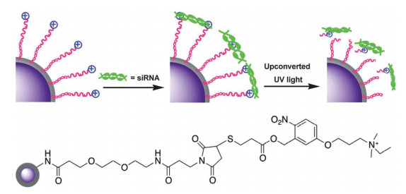
Niikura K, Kobayashi K, Takeuchi C, et al. (2014) Amphiphilic gold nanoparticles displaying flexible bifurcated ligands as a carrier for siRNA delivery into the cell cytosol. ACS Appl Mater Interfaces 6: 22146–22154. doi: 10.1021/am505577j
    [7] Yamashita S, Fukushima H, Niidome Y, et al. (2011) Controlled-release system mediated by a retro Diels-Alder reaction induced by the photothermal effect of gold nanorods. Langmuir 27: 14621–14626. doi: 10.1021/la2036746
    [8] Neumann K, Jain S, Geng J, et al. (2016) Nanoparticle "switch-on" by tetrazine triggering. Chem Commun 52: 11223–11226. doi: 10.1039/C6CC05118A
    [9] Zhang P, He Z, Wang C, et al. (2015) In situ amplification of intracellular microRNA with MNazyme nanodevices for multiplexed imaging, logic operation, and controlled drug release. ACS Nano 9: 789–798. doi: 10.1021/nn506309d
    [10] Shakiba A, Jamison AC, Lee TR (2015) Poly(L-lysine) interfaces via dual click reactions on surface-bound custom-designed dithiol adsorbates. Langmuir 31: 6154–6163. doi: 10.1021/acs.langmuir.5b00877
    [11] Nuzzo RG, Allara DL (1983) Adsorption of bifunctional organic disulfides on gold surfaces. J Am Chem Soc 105: 4481–4483. doi: 10.1021/ja00351a063
    [12] Bain CD, Whitesides GM (1988) Correlations between wettability and structure in monolayers of alkanethiols adsorbed on gold. J Am Chem Soc 110: 3665–3666. doi: 10.1021/ja00219a055
    [13] Bain CD, Troughton EB, Tao YT, et al. (1989) Formation of monolayer films by the spontaneous assembly of organic thiols from solution onto gold. J Am Chem Soc 111: 321–335. doi: 10.1021/ja00183a049
    [14] Irving DL, Brenner DW (2006) Diffusion on a self-assembled monolayer:  molecular modeling of a bound + mobile lubricant. J Phys Chem B 110: 15426–15431. doi: 10.1021/jp0609840
    [15] Xiang HY, Li WG (2009) Electrochemical sensor for trans-resveratrol determination based on indium tin oxide electrode modified with molecularly imprinted self-assembled films. Electroanalysis 21: 1207–1210. doi: 10.1002/elan.200804488
    [16] Li S, Yang D, Tu H, et al. (2013) Protein adsorption and cell adhesion controlled by the surface chemistry of binary perfluoroalkyl/oligo(ethylene glycol) self-assembled monolayers. J Colloid Interface Sci 402: 284–290. doi: 10.1016/j.jcis.2013.04.003
    [17] Wolf LK, Fullenkamp DE, Georgiadis RM (2005) Quantitative angle-resolved SPR imaging of DNA-DNA and DNA-drug kinetics. J Am Chem Soc 127: 17453–17459. doi: 10.1021/ja056422w
    [18] Love JC, Estroff LA, Kriebel JK, et al. (2005) Self-assembled monolayers of thiolates on metals as a form of nanotechnology. Chem Rev 105: 1103–1170. doi: 10.1021/cr0300789
    [19] Crudden CM, Horton JH, Ebralidze II, et al. (2014) Ultra stable self-assembled monolayers of N-heterocyclic carbenes on gold. Nat Chem 6: 409–414. doi: 10.1038/nchem.1891
    [20] Cao C, Kim JP, Kim BW, et al. (2006) A strategy for sensitivity and specificity enhancements in prostate specific antigen-1-antichymotrypsin detection based on surface plasmon resonance. Biosens Bioelectron 21: 2106–2113. doi: 10.1016/j.bios.2005.10.014
    [21] Khantamat O, Li CH, Yu F, et al. (2015) Gold nanoshell-decorated silicone surfaces for the near-infrared (NIR) photothermal destruction of the pathogenic bacterium E. faecalis. ACS Appl Mater Interfaces 7: 3981–3993. doi: 10.1021/am506516r
    [22] Huang CJ, Chen YS, Chang Y (2015) Counterion-activated nanoactuator: reversibly switchable killing/releasing bacteria on polycation brushes. ACS Appl Mater Interfaces 7: 2415–2423. doi: 10.1021/am507105r
    [23] Ilyas S, Ilyas M, Van der Hoorn RAL, et al. (2013) Selective conjugation of proteins by mining active proteomes through click-functionalized magnetic nanoparticles. ACS Nano 7: 9655–9663. doi: 10.1021/nn402382g
    [24] Farokhzad OC, Langer R (2009) Impact of nanotechnology on drug delivery. ACS Nano 3: 16–20. doi: 10.1021/nn900002m
    [25] Zhang J, Fu Y, Mei Y, et al. (2010) Fluorescent metal nanoshell probe to detect single miRNA in lung cancer cell. Anal Chem 82: 4464–4471. doi: 10.1021/ac100241f
    [26] Latham AH, Williams ME (2006) Versatile routes toward functional, water-soluble nanoparticles via trifluoroethylester-PEG-thiol ligands. Langmuir 22: 4319–4326. doi: 10.1021/la053523z
    [27] Gentilini C, Evangelista F, Rudolf P, et al. (2008) Water-soluble gold nanoparticles protected by fluorinated amphiphilic thiolates. J Am Chem Soc 130: 15678–15682. doi: 10.1021/ja8058364
    [28] Salvati A, Pitek AS, Monopoli MP, et al. (2013) Transferrin-functionalized nanoparticles lose their targeting capabilities when a biomolecule corona adsorbs on the surface. Nat Nanotechnol 8: 137–143. doi: 10.1038/nnano.2012.237
    [29] Krafft MP, Riess JG (2007) Perfluorocarbons: life sciences and biomedical uses dedicated to the memory of Professor Guy Ourisson, a true renaissance man. J Polym Sci Part A: Polym Chem 45: 1185–1198. doi: 10.1002/pola.21937
    [30] Frotscher E, Danielczak B, Vargas C, et al. (2015) A fluorinated detergent for membrane-protein applications. Angew Chem Int Ed 54: 5069–5073. doi: 10.1002/anie.201412359
    [31] Kurczy ME, Zhu ZJ, Ivanisevic J, et al. (2015) Comprehensive bioimaging with fluorinated nanoparticles using breathable liquids. Nat Commun 6: 5998–6003. doi: 10.1038/ncomms6998
    [32] Ogawa M, Nitahara S, Aoki H, et al. (2010) Synthesis and evaluation of water-soluble fluorinated dendritic block-copolymer nanoparticles as a 19F-MRI contrast agent. Macromol Chem Phys 211: 1602–1609. doi: 10.1002/macp.201000100
    [33] McIntosh CM, Esposito EA, Boal AK, et al. (2001) Inhibition of DNA transcription using cationic mixed monolayer protected gold clusters. J Am Chem Soc 123: 7626–7629. doi: 10.1021/ja015556g
    [34] Li F, Zhang H, Dever B, et al. (2013) Thermal stability of DNA functionalized gold nanoparticles. Bioconjugate Chem 24: 1790–1797. doi: 10.1021/bc300687z
    [35] Liu X, Huang H, Jin Q, et al. (2011) Mixed charged zwitterionic self-assembled monolayers as a facile way to stabilize large gold nanoparticles. Langmuir 27: 5242–5251. doi: 10.1021/la2002223
    [36] Li H, Liu X, Huang N, et al. (2014) "Mixed-charge self-assembled monolayers" as a facile method to design pH-induced aggregation of large gold nanoparticles for near-infrared photothermal cancer therapy. ACS Appl Mater Interfaces 6: 18930–18937. doi: 10.1021/am504813f
    [37] Liu X, Chen Y, Li H, et al. (2013) Enhanced retention and cellular uptake of nanoparticles in tumors by controlling their aggregation behavior. ACS Nano 7: 6244–6257. doi: 10.1021/nn402201w
    [38] Nair DP, Podgórski M, Chatani S, et al. (2014) The thiol-Michael addition click reaction: a powerful and widely used tool in materials chemistry. Chem Mater 26: 724–744. doi: 10.1021/cm402180t
    [39] Luedtke WD, Landman U (1996) Structure, dynamics, and thermodynamics of passivated gold nanocrystallites and their assemblies. J Phys Chem 100: 13323–13329. doi: 10.1021/jp961721g
    [40] Goulet PJG, Lennox RB (2010) New insights into brust-schiffrin metal nanoparticle synthesis. J Am Chem Soc 132: 9582–9584. doi: 10.1021/ja104011b
    [41] Chang WC, Tai JT, Wang HF, et al. (2016) Surface PEGylation of silver nanoparticles: kinetics of simultaneous surface dissolution and molecular desorption. Langmuir 32: 9807–9815. doi: 10.1021/acs.langmuir.6b02338
    [42] Cargnello M, Wieder NL, Canton P, et al. (2011) A versatile approach to the synthesis of functionalized thiol-protected palladium nanoparticles. Chem Mater 23: 3961–3969. doi: 10.1021/cm2014658
    [43] Mei BC, Susumu K, Medintz IL, et al. (2008) Modular poly(ethylene glycol) ligands for biocompatible semiconductor and gold nanocrystals with extended ph and ionic stability. J Mater Chem 18: 4949–4958. doi: 10.1039/b810488c
    [44] Brust M, Walker M, Bethell D, et al. (1994) Synthesis of thiol-derivatised gold nanoparticles in a two-phase liquid-liquid system. J Chem Soc Chem Commun 7: 801–802.
    [45] Hong R, Fischer NO, Verma A, et al. (2004) Control of protein structure and function through surface recognition by tailored nanoparticle scaffolds. J Am Chem Soc 126: 739–743. doi: 10.1021/ja037470o
    [46] Zenasni O, Jamison AC, Lee TR (2013) The impact of fluorination on the structure and properties of self-assembled monolayer films. Soft Matter 9: 6356–6370. doi: 10.1039/c3sm00054k
    [47] Lee HJ, Jamison AC, Yuan Y, et al. (2013) Robust carboxylic acid-terminated organic thin films and nanoparticle protectants generated from bidentate alkanethiols. Langmuir 29: 10432–10439. doi: 10.1021/la4017118
    [48] Zhang S, Leem G, Srisombat LO, et al. (2008) Rationally designed ligands that inhibit the aggregation of large gold nanoparticles in solution. J Am Chem Soc 130: 113–120. doi: 10.1021/ja0724588
    [49] Chinwangso P, Jamison AC, Lee TR (2011) Multidentate adsorbates for self-assembled monolayer films. Acc Chem Res 44: 511–519. doi: 10.1021/ar200020s
    [50] Srisombat LO, Zhang S, Lee TR (2010) Thermal stability of mono-, bis-, and tris-chelating alkanethiol films assembled on gold nanoparticles and evaporated "flat" gold. Langmuir 26: 41–46. doi: 10.1021/la902082j
    [51] Jacquelín DK, Pérez MA, Euti EM, et al. (2016) A pH-sensitive supramolecular switch based on mixed carboxylic acid terminated self-assembled monolayers on Au(111). Langmuir 32: 947–953. doi: 10.1021/acs.langmuir.5b03807
    [52] Lai SF, Tan HR, Tok ES, et al. (2015) Optimization of gold nanoparticle photoluminescence by alkanethiolation. Chem Commun 51: 7954–7957. doi: 10.1039/C5CC01229E
    [53] Stiti M, Cecchi A, Rami M, et al. (2008) Carbonic anhydrase inhibitor coated gold nanoparticles selectively inhibit the tumor-associated isoform ix over the cytosolic isozymes I and II. J Am Chem Soc 130: 16130–16131. doi: 10.1021/ja805558k
    [54] Burns CJ, Field LD, Petteys BJ, et al. (2005) Synthesis and characterization of sams and tethered bilayer membranes from unsymmetrically substituted 1,2-dithianes. Aust J Chem 58: 738–748. doi: 10.1071/CH05175
    [55] Shon YS, Lee S, Perry SS, et al. (2000) The adsorption of unsymmetrical spiroalkanedithiols onto gold affords multi-component interfaces that are homogeneously mixed at the molecular level. J Am Chem Soc 122: 1278–1281. doi: 10.1021/ja991987b
    [56] Chinwangso P, Lee HJ, Lee TR (2015) Self-assembled monolayers generated from unsymmetrical partially fluorinated spiroalkanedithiols. Langmuir 31: 13341–13349. doi: 10.1021/acs.langmuir.5b03392
    [57] Sabatani E, Cohen BJ, Bruening M, et al. (1993) Thioaromatic monolayers on gold: a new family of self-assembling monolayers. Langmuir 9: 2974–2981. doi: 10.1021/la00035a040
    [58] Bruno G, Babudri F, Operamolla A, et al. (2010) Tailoring density and optical and thermal behavior of gold surfaces and nanoparticles exploiting aromatic dithiols. Langmuir 26: 8430–8440. doi: 10.1021/la101082t
    [59] Sano KI, Shiba K (2003) A hexapeptide motif that electrostatically binds to the surface of titanium. J Am Chem Soc 125: 14234–14235. doi: 10.1021/ja038414q
    [60] Gabriel M, Nazmi K, Veerman EC, et al. (2006) Preparation of LL-37-grafted titanium surfaces with bactericidal activity. Bioconjugate Chem 17: 548–550. doi: 10.1021/bc050091v
    [61] Haynie SL, Crum GA, Doele BA (1995) Antimicrobial activities of amphiphilic peptides covalently bonded to a water-insoluble resin. Antimicrob Agents Chemother 39: 301–307. doi: 10.1128/AAC.39.2.301
    [62] Yoon HJ, Kim TH, Zhang Z, et al. (2013) Sensitive capture of circulating tumour cells by functionalized graphene oxide nanosheets. Nat Nanotechnol 8: 735–741. doi: 10.1038/nnano.2013.194
    [63] Haasnoot J, Westerhout EM, Berkhout B (2007) RNA interference against viruses: strike and counterstrike. Nat Biotechnol 25: 1435–1443. doi: 10.1038/nbt1369
    [64] Castanotto D, Rossi JJ (2009) The promises and pitfalls of RNA-interference-based therapeutics. Nature 457: 426–433. doi: 10.1038/nature07758
    [65] Torchilin VP, Lukyanov AN, Gao Z, et al. (2003) Immunomicelles: targeted pharmaceutical carriers for poorly soluble drugs. Proc Natl Acad Sci USA 100: 6039–6044. doi: 10.1073/pnas.0931428100
    [66] Conde J, Ambrosone A, Sanz V, et al. (2012) Design of multifunctional gold nanoparticles for in vitro and in vivo gene silencing. ACS Nano 6: 8316–8324. doi: 10.1021/nn3030223
    [67] Rosi NL, Giljohann DA, Thaxton CS, et al. (2006) Oligonucleotide-modified gold nanoparticles for intracellular gene regulation. Science 312: 1027–1030. doi: 10.1126/science.1125559
    [68] Loh XJ, Lee TC, Dou Q, et al. (2016) Utilising inorganic nanocarriers for gene delivery. Biomater Sci 4: 70–86. doi: 10.1039/C5BM00277J
    [69] Tan SJ, Kiatwuthinon P, Roh YH, et al. (2011) Engineering nanocarriers for siRNA delivery. Small 7: 841–856. doi: 10.1002/smll.201001389
    [70] Miele E, Spinelli GP, Miele E, et al. (2012) Nanoparticle-based delivery of small interfering rna: challenges for cancer therapy. Int J Nanomed 7: 3637–3657.
    [71] Wijaya A, Schaffer SB, Pallares IG, et al. (2009) Selective release of multiple DNA oligonucleotides from gold nanorods. ACS Nano 3: 80–86. doi: 10.1021/nn800702n
    [72] Braun GB, Pallaoro A, Wu G, et al. (2009) Laser-activated gene silencing via gold nanoshell-sirna conjugates. ACS Nano 3: 2007–2015. doi: 10.1021/nn900469q
    [73] Doane T, Burda C (2013) Nanoparticle mediated non-covalent drug delivery. Adv Drug Deliv Rev 65: 607–621. doi: 10.1016/j.addr.2012.05.012
    [74] Alexis F, Pridgen E, Molnar LK, et al. (2008) Factors affecting the clearance and biodistribution of polymeric nanoparticles. Mol Pharm 5: 505–515. doi: 10.1021/mp800051m
    [75] Warrington R (2012) Drug allergy: causes and desensitization. Hum Vacc Immunother 8: 1513–1524.
    [76] Kim HJ, Miyata K, Nomoto T, et al. (2014) siRNA delivery from triblock copolymer micelles with spatially-ordered compartments of PEG shell, siRNA-loaded intermediate layer, and hydrophobic core. Biomaterials 35: 4548–4556. doi: 10.1016/j.biomaterials.2014.02.016
    [77] Ortac I, Simberg D, Yeh YS, et al. (2014) Dual-porosity hollow nanoparticles for the immunoprotection and delivery of nonhuman enzymes. Nano Lett 14: 3023–3032. doi: 10.1021/nl404360k
    [78] Han L, Zhao J, Zhang X, et al. (2012) Enhanced siRNA delivery and silencing gold-chitosan nanosystem with surface charge-reversal polymer assembly and good biocompatibility. ACS Nano 6: 7340–7351. doi: 10.1021/nn3024688
    [79] Wu Z, Liu GQ, Yang XL, et al. (2015) Electrostatic nucleic acid nanoassembly enables hybridization chain reaction in living cells for ultrasensitive mRNA imaging. J Am Chem Soc 137: 6829–6836. doi: 10.1021/jacs.5b01778
    [80] Guo S, Huang Y, Jiang Q, et al. (2010) Enhanced gene delivery and siRNA silencing by gold nanoparticles coated with charge-reversal polyelectrolyte. ACS Nano 4: 5505–5511. doi: 10.1021/nn101638u
    [81] Lin J, Zhang H, Chen Z, et al. (2010) Penetration of lipid membranes by gold nanoparticles: insights into cellular uptake, cytotoxicity, and their relationship. ACS Nano 4: 5421–5429. doi: 10.1021/nn1010792
    [82] Oh N, Park JH (2014) Endocytosis and exocytosis of nanoparticles in mammalian cells. Int J Nanomed 1: 51–63.
    [83] Zhang Y, Kohler N, Zhang M (2002) Surface modification of superparamagnetic magnetite nanoparticles and their intracellular uptake. Biomaterials 23: 1553–1561. doi: 10.1016/S0142-9612(01)00267-8
    [84] Van Dam GM, Themelis G, Crane LMA, et al. (2011) Intraoperative tumor-specific fluorescence imaging in ovarian cancer by folate receptor-[alpha] targeting: first in-human results. Nat Med 17: 1315–1319. doi: 10.1038/nm.2472
    [85] Ma K, Wang DD, Lin Y, et al. (2013) Synergetic targeted delivery of sleeping-beauty transposon system to mesenchymal stem cells using lpd nanoparticles modified with a phage-displayed targeting peptide. Adv Funct Mater 23: 1172–1181. doi: 10.1002/adfm.201102963
    [86] Chang B, Sha X, Guo J, et al. (2011) Thermo and pH dual responsive, polymer shell coated, magnetic mesoporous silica nanoparticles for controlled drug release. J Mater Chem 21: 9239–9247. doi: 10.1039/c1jm10631g
    [87] Zhang MH, Gu ZP, Zhang X, et al. (2015) pH-sensitive ternary nanoparticles for nonviral gene delivery. Rsc Adv 5: 44291–44298. doi: 10.1039/C5RA04745E
    [88] Vander HMG, Cantley LC, Thompson CB (2009) Understanding the Warburg effect: the metabolic requirements of cell proliferation. Science 324: 1029–1033. doi: 10.1126/science.1160809
    [89] Lu J, Tan M, Cai Q (2015) The Warburg effect in tumor progression: mitochondrial oxidative metabolism as an anti-metastasis mechanism. Cancer Lett 356: 156–164. doi: 10.1016/j.canlet.2014.04.001
    [90] Muhammad F, Wang A, Guo M, et al. (2013) pH dictates the release of hydrophobic drug cocktail from mesoporous nanoarchitecture. ACS Appl Mater Interfaces 5: 11828–11835. doi: 10.1021/am4035027
    [91] Lin Q, Bao C, Cheng S, et al. (2012) Target-activated coumarin phototriggers specifically switch on fluorescence and photocleavage upon bonding to thiol-bearing protein. J Am Chem Soc 134: 5052–5055. doi: 10.1021/ja300475k
    [92] Brown PK, Qureshi AT, Moll AN, et al. (2013) Silver nanoscale antisense drug delivery system for photoactivated gene silencing. ACS Nano 7: 2948–2959. doi: 10.1021/nn304868y
    [93] Il'ichev YV, Schwörer MA, Wirz J (2004) Photochemical reaction mechanisms of 2-nitrobenzyl compounds:  methyl ethers and caged ATP. J Am Chem Soc 126: 4581–4595. doi: 10.1021/ja039071z
    [94] Han G, You CC, Kim BJ, et al. (2006) Light-regulated release of dna and its delivery to nuclei by means of photolabile gold nanoparticles. Angew Chem Int Ed 45: 3165–3169. doi: 10.1002/anie.200600214
    [95] Weissleder R (2001) A clearer vision for in vivo imaging. Nat Biotech 19: 316–317. doi: 10.1038/86684
    [96] Liu Q, Sun Y, Yang T, et al. (2011) Sub-10 nm hexagonal lanthanide-doped NaLuF4 upconversion nanocrystals for sensitive bioimaging in vivo. J Am Chem Soc 133: 17122–17125. doi: 10.1021/ja207078s
    [97] Jaque D, Martinez ML, del Rosal B, et al. (2014) Nanoparticles for photothermal therapies. Nanoscale 6: 9494–9530. doi: 10.1039/C4NR00708E
    [98] Zhao L, Peng J, Huang Q, et al. (2014) Near-infrared photoregulated drug release in living tumor tissue via yolk-shell upconversion nanocages. Adv Funct Mater 24: 363–371. doi: 10.1002/adfm.201302133
    [99] Yang Y, Liu F, Liu X, et al. (2013) NIR light controlled photorelease of sirna and its targeted intracellular delivery based on upconversion nanoparticles. Nanoscale 5: 231–238. doi: 10.1039/C2NR32835F
    [100] Huang X, El-Sayed MA (2010) Gold nanoparticles: optical properties and implementations in cancer diagnosis and photothermal therapy. J Adv Res 1: 13–28. doi: 10.1016/j.jare.2010.02.002
    [101] 
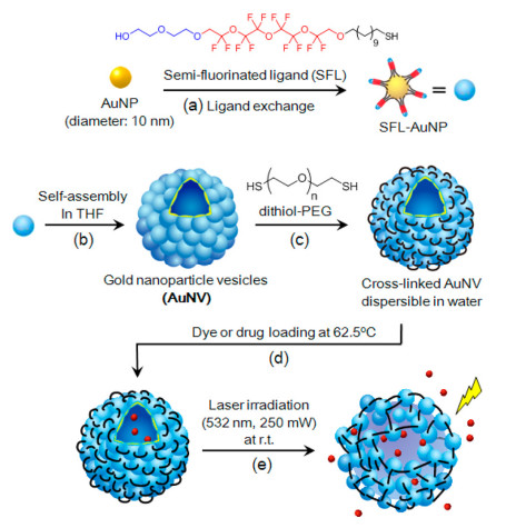
Niikura K, Iyo N, Matsuo Y, et al. (2013) Sub-100 nm gold nanoparticle vesicles as a drug delivery carrier enabling rapid drug release upon light irradiation. ACS Appl Mater Interfaces 5: 3900–3907. doi: 10.1021/am400590m
    [102] Niikura K, Iyo N, Higuchi T, et al. (2012) Gold nanoparticles coated with semi-fluorinated oligo(ethylene glycol) produce sub-100 nm nanoparticle vesicles without templates. J Am Chem Soc 134: 7632–7635. doi: 10.1021/ja302122w
    [103] Zhang Z, Wang J, Nie X, et al. (2014) Near infrared laser-induced targeted cancer therapy using thermoresponsive polymer encapsulated gold nanorods. J Am Chem Soc 136: 7317–7326. doi: 10.1021/ja412735p
    [104] 
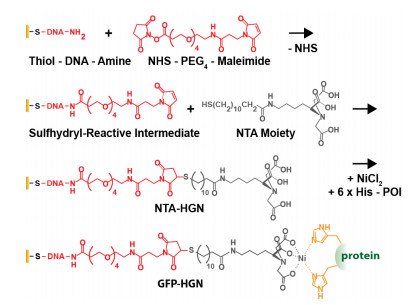
Morales DP, Braun GB, Pallaoro A, et al. (2015) Targeted intracellular delivery of proteins with spatial and temporal control. Mol Pharm 12: 600–609. doi: 10.1021/mp500675p
    [105] 
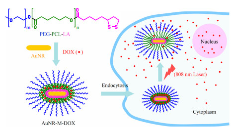
Zhong Y, Wang C, Cheng L, et al. (2013) Gold nanorod-cored biodegradable micelles as a robust and remotely controllable doxorubicin release system for potent inhibition of drug-sensitive and -resistant cancer cells. Biomacromolecules 14: 2411–2419. doi: 10.1021/bm400530d
    [106] Jones ST, Walsh KZ, Barrow SJ, et al. (2016) The importance of excess poly(n-isopropylacrylamide) for the aggregation of poly(n-isopropylacrylamide)-coated gold nanoparticles. ACS Nano 10: 3158–3165. doi: 10.1021/acsnano.5b04083
    [107] Yavuz MS, Cheng Y, Chen J, et al. (2009) Gold nanocages covered by smart polymers for controlled release with near-infrared light. Nat Mater 8: 935–939. doi: 10.1038/nmat2564
    [108] Roy D, Brooks WLA, Sumerlin BS (2013) New directions in thermoresponsive polymers. Chem Soc Rev 42: 7214–7243. doi: 10.1039/c3cs35499g
    [109] Thomas CR, Ferris DP, Lee JH, et al. (2010) Noninvasive remote-controlled release of drug molecules in vitro using magnetic actuation of mechanized nanoparticles. J Am Chem Soc 132: 10623–10625. doi: 10.1021/ja1022267
    [110] Choi SW, Zhang Y, Xia Y (2010) A temperature-sensitive drug release system based on phase-change materials. Angew Chem Int Ed 49: 7904–7908. doi: 10.1002/anie.201004057
    [111] Tian L, Gandra N, Singamaneni S (2013) Monitoring controlled release of payload from gold nanocages using surface enhanced raman scattering. ACS Nano 7: 4252–4260. doi: 10.1021/nn400728t
    [112] Jia X, Cai X, Chen Y, et al. (2015) Perfluoropentane-encapsulated hollow mesoporous prussian blue nanocubes for activated ultrasound imaging and photothermal therapy of cancer. ACS Appl Mater Interfaces 7: 4579–4588. doi: 10.1021/am507443p
    [113] Moon GD, Choi SW, Cai X, et al. (2011) A new theranostic system based on gold nanocages and phase-change materials with unique features for photoacoustic imaging and controlled release. J Am Chem Soc 133: 4762–4765. doi: 10.1021/ja200894u
    [114] 
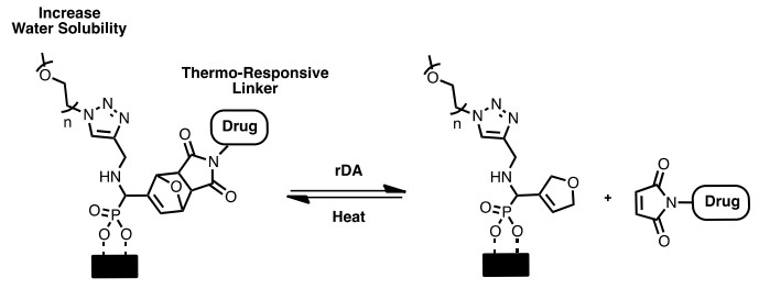
Zhu J, Kell AJ, Workentin MS (2006) A retro-Diels-Alder reaction to uncover maleimide-modified surfaces on monolayer-protected nanoparticles for reversible covalent assembly. Org Lett 8: 4993–4996. doi: 10.1021/ol0615937
    [115] Hammad M, Nica V, Hempelmann R (2017) On-command controlled drug release by Diels-Alder reaction using bi-magnetic core/shell nano-carriers. Colloid Surf B 150: 15–22. doi: 10.1016/j.colsurfb.2016.11.005
    [116] N'Guyen TTT, Duong HTT, Basuki J, et al. (2013) Functional iron oxide magnetic nanoparticles with hyperthermia-induced drug release ability by using a combination of orthogonal click reactions. Angew Chem Int Ed 52: 14152–14156. doi: 10.1002/anie.201306724
    [117] Kolhatkar A, Jamison A, Litvinov D, et al. (2013) Tuning the magnetic properties of nanoparticles. Int J Mol Sci 14: 15977–16009. doi: 10.3390/ijms140815977
    [118] 
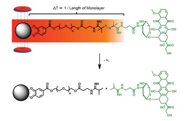
Riedinger A, Guardia P, Curcio A, et al. (2013) Subnanometer local temperature probing and remotely controlled drug release based on azo-functionalized iron oxide nanoparticles. Nano Lett 13: 2399–2406. doi: 10.1021/nl400188q
  • This article has been cited by:

    1. Nguyen Thi Thu Thuy, Tran Thanh Tung, Strong convergence of one-step inertial algorithm for a class of bilevel variational inequalities, 2025, 0233-1934, 1, 10.1080/02331934.2024.2448737
    2. Nguyen Thi Thu Thuy, Tran Thanh Tung, Le Xuan Ly, Strongly convergent two-step inertial algorithm for a class of bilevel variational inequalities, 2025, 44, 2238-3603, 10.1007/s40314-024-03078-7
    3. Le Xuan Ly, Nguyen Thi Thu Thuy, Nguyen Quoc Anh, Relaxed two-step inertial method for solving a class of split variational inequality problems with application to traffic analysis, 2025, 0233-1934, 1, 10.1080/02331934.2025.2459191
  • Reader Comments
  • © 2017 the Author(s), licensee AIMS Press. This is an open access article distributed under the terms of the Creative Commons Attribution License (http://creativecommons.org/licenses/by/4.0)
通讯作者: 陈斌, bchen63@163.com
  • 1. 

    沈阳化工大学材料科学与工程学院 沈阳 110142

  1. 本站搜索
  2. 百度学术搜索
  3. 万方数据库搜索
  4. CNKI搜索

Metrics

Article views(9859) PDF downloads(1829) Cited by(17)

/

DownLoad:  Full-Size Img  PowerPoint
Return
Return

Catalog