
Citation: James L. Gole. Nanostructured metal oxide modification of a porous silicon interface for sensor applications: the question of water interaction, stability, platform diversity and sensitivity, and selectivity[J]. AIMS Electronics and Electrical Engineering, 2020, 4(1): 87-113. doi: 10.3934/ElectrEng.2020.1.87
[1] | Yves Achdou, Ziad Kobeissi . Mean field games of controls: Finite difference approximations. Mathematics in Engineering, 2021, 3(3): 1-35. doi: 10.3934/mine.2021024 |
[2] | Benoît Perthame, Edouard Ribes, Delphine Salort . Career plans and wage structures: a mean field game approach. Mathematics in Engineering, 2019, 1(1): 38-54. doi: 10.3934/Mine.2018.1.38 |
[3] | Piermarco Cannarsa, Rossana Capuani, Pierre Cardaliaguet . C1;1-smoothness of constrained solutions in the calculus of variations with application to mean field games. Mathematics in Engineering, 2019, 1(1): 174-203. doi: 10.3934/Mine.2018.1.174 |
[4] | Pablo Blanc, Fernando Charro, Juan J. Manfredi, Julio D. Rossi . Games associated with products of eigenvalues of the Hessian. Mathematics in Engineering, 2023, 5(3): 1-26. doi: 10.3934/mine.2023066 |
[5] | Simone Paleari, Tiziano Penati . Hamiltonian lattice dynamics. Mathematics in Engineering, 2019, 1(4): 881-887. doi: 10.3934/mine.2019.4.881 |
[6] | Mario Pulvirenti . On the particle approximation to stationary solutions of the Boltzmann equation. Mathematics in Engineering, 2019, 1(4): 699-714. doi: 10.3934/mine.2019.4.699 |
[7] | Franco Flandoli, Eliseo Luongo . Heat diffusion in a channel under white noise modeling of turbulence. Mathematics in Engineering, 2022, 4(4): 1-21. doi: 10.3934/mine.2022034 |
[8] | Giacomo Canevari, Arghir Zarnescu . Polydispersity and surface energy strength in nematic colloids. Mathematics in Engineering, 2020, 2(2): 290-312. doi: 10.3934/mine.2020015 |
[9] | Zheming An, Nathaniel J. Merrill, Sean T. McQuade, Benedetto Piccoli . Equilibria and control of metabolic networks with enhancers and inhibitors. Mathematics in Engineering, 2019, 1(3): 648-671. doi: 10.3934/mine.2019.3.648 |
[10] | Jérôme Droniou, Jia Jia Qian . Two arbitrary-order constraint-preserving schemes for the Yang–Mills equations on polyhedral meshes. Mathematics in Engineering, 2024, 6(3): 468-493. doi: 10.3934/mine.2024019 |
The authors are honored to participate in this special issue and express their admiration to Professor Italo Capuzzo-Dolcetta for his mathematical work. The first author met Prof. Dolcetta for the first time at the end of his Ph.D. thesis more than 20 years ago during an extended visit to Roma. Prof. Dolcetta mentorship at that time influenced his career deeply and he is particularly grateful for this opportunity.
Mean-field games (MFG) is a tool to study the Nash equilibrium of infinite populations of rational agents. These agents select their actions based on their state and the statistical information about the population. Here, we study a price formation model for a commodity traded in a market under uncertain supply, which is a common noise shared by the agents. These agents are rational and aim to minimize the average trading cost by selecting their trading rate. The distribution of the agents solves a stochastic partial differential equation. Finally, a market-clearing condition characterizes the price.
We let (Ω,F,(Ft)0⩽t,P) be a complete filtered probability space such that (Ft)0⩽t is the standard filtration induced by t↦Wt, the common noise, which is a one-dimensional Brownian motion. We consider a commodity whose supply process is described by a stochastic differential equation; that is, we are given a drift bS:[0,T]×R2→R and volatility σS:[0,T]×R2→R+0, which are smooth functions, and the supply Qs is determined by the stochastic differential equation
dQs=bS(Qs,ϖs,s)ds+σS(Qs,ϖs,s)dWs in [0,T] | (1.1) |
with the initial condition ˉq. We would like to determine the drift bP:[0,T]×R2→R, the volatility σP:[0,T]×R2→R+0, and ˉw such that the price ϖs solves
dϖs=bP(Qs,ϖs,s)ds+σP(Qs,ϖs,s)dWs in [0,T] | (1.2) |
with initial condition ˉw and such that it ensures a market clearing condition. It may not be possible to find bP and σP in a feedback form. However, for linear dynamics, as we show here, we can solve quadratic models, which are of great interest in applications.
Let Xs be the quantity of the commodity held by an agent at time s for t⩽s⩽T. This agent trades this commodity, controlling its rate of change, v, thus
dXs=v(s)ds in [t,T]. | (1.3) |
At time t, an agent who holds x and observes q and w chooses a control process v, progressively measurable with respect to Ft, to minimize the expected cost functional
J(x,q,w,t;v)=E[∫TtL(Xs,v(s))+ϖsv(s)ds+Ψ(XT,QT,ϖT)], | (1.4) |
subject to the dynamics (1.1), (1.2), and (1.3) with initial condition Xt=x, and the expectation is taken w.r.t. Fr. The Lagrangian, L, takes into account costs such as market impact or storage, and the terminal cost Ψ stands for the terminal preferences of the agent.
This control problem determines a Hamilton-Jacobi equation addressed in Section 2.1. In turn, each agent selects an optimal control and uses it to adjust its holdings. Because the source of noise in Qt is common to all agents, the evolution of the probability distribution of agents is not deterministic. Instead, it is given by a stochastic transport equation derived in Section 2.2. Finally, the price is determined by a market-clearing condition that ensures that supply meets demand. We study this condition in Section 2.3.
Mathematically, the price model corresponds to the following problem.
Problem 1. Given a Hamiltonian, H:R2→R, H∈C∞, a commodity's supply initial value, ˉq∈R, supply drift, bS:R2×[0,T]→R, and supply volatility, σS:R2×[0,T]→R, a terminal cost, Ψ:R3→R, Ψ∈C∞(R3), and an initial distribution of agents, ˉm∈C∞c(R)∩P(R), find u:R3×[0,T]→R, μ∈C([0,T]×Ω;P(R3)), ˉw∈R, the price at t=0, the price drift bP:R2×[0,T]→R, and the price volatility σP:R2×[0,T]→R solving
{−ut+H(x,w+ux)=bSuq+bPuw+12(σS)2uqq+σSσPuqw+12(σP)2uwwdμt=((μ(σS)22)qq+(μσSσP)qw+(μ(σP)22)ww−div(μb))dt−div(μσ)dWt∫R3q+DpH(x,w+ux(x,q,w,t))μt(dx×dq×dw)=0,a.e.ω∈Ω,0⩽t⩽T, | (1.5) |
and the terminal-initial conditions
{u(x,q,w,T)=Ψ(x,q,w)μ0=ˉm×δˉq×δˉw, | (1.6) |
where b=(−DpH(x,w+ux),bS,bP), σ=(0,σS,σP), and the divergence is taken w.r.t. (x,q,w).
Given a solution to the preceding problem, we construct the supply and price processes
Qt=∫R3qμt(dx×dq×dw) |
and
ϖt=∫R3wμt(dx×dq×dw), |
which also solve
{dQt=bS(Qt,ϖt,t)dt+σS(Qt,ϖt,t)dWt in [0,T]dϖt=bP(Qt,ϖt,t)dt+σP(Qt,ϖt,t)dWt in [0,T] |
with initial conditions
{Q0=ˉqϖ0=ˉw | (1.7) |
and satisfy the market-clearing condition
Qt=∫R−DpH(x,ϖt+ux(x,Qt,ϖt,t))μt(dx). |
In [10], the authors presented a model where the supply for the commodity was a given deterministic function, and the balance condition between supply and demand gave rise to the price as a Lagrange multiplier. Price formation models were also studied by Markowich et al. [18], Caffarelli et al. [2], and Burger et al. [1]. The behavior of rational agents that control an electric load was considered in [16,17]. For example, turning on or off space heaters controls the electric load as was discussed in [13,14,15]. Previous authors addressed price formation when the demand is a given function of the price [12] or that the price is a function of the demand, see, for example [5,6,7,8,11]. An N-player version of an economic growth model was presented in [9].
Noise in the supply together with a balance condition is a central issue in price formation that could not be handled directly with the techniques in previous papers. A probabilistic approach of the common noise is discussed in Carmona et al. in [4]. Another approach is through the master equation, involving derivatives with respect to measures, which can be found in [3]. None of these references, however, addresses problems with integral constraints such as (1.7).
Our model corresponds to the one in [10] for the deterministic setting when we take the volatility for the supply to be 0. Here, we study the linear-quadratic case, that is, when the cost functional is quadratic, and the dynamics (1.1) and (1.2) are linear. In Section 3.2, we provide a constructive approach to get semi-explicit solutions of price models for linear dynamics and quadratic cost. This approach avoids the use of the master equation. The paper ends with a brief presentation of simulation results in Section 4.
In this section, we derive Problem 1 from the price model. We begin with standard tools of optimal control theory. Then, we derive the stochastic transport equation, and we end by introducing the market-clearing (balance) condition.
The value function for an agent who at time t holds an amount x of the commodity, whose instantaneous supply and price are q and w, is
u(x,q,w,t)=inf | (2.1) |
where J is given by (1.4) and the infimum is taken over the set {\mathcal{A}}\left((t, T]\right) of all functions v:[t, T]\to {\mathbb{R}} , progressively measurable w.r.t. (\mathcal{F}_s)_{t{\leqslant} s {\leqslant} T} . Consider the Hamiltonian, H , which is the Legendre transform of L ; that is, for p\in {\mathbb{R}} ,
\begin{equation} H(x, p) = \sup\limits_{v\in {\mathbb{R}}} [-pv-L (x, v)]. \end{equation} | (2.2) |
Then, from standard stochastic optimal control theory, whenever L is strictly convex, if u is C^2 , it solves the Hamilton-Jacobi equation in {\mathbb{R}}^3 \times [0, T)
\begin{equation} -u_t+H(x, w+u_x) -b^Pu_w -b^S u_q - \tfrac{(\sigma^P)^2}{2}u_{ww}- \tfrac{(\sigma^S)^2}{2}u_{qq}- \sigma^P\sigma^Su_{wq} = 0 \end{equation} | (2.3) |
with the terminal condition
\begin{equation} u(x, q, w, T) = \Psi \left(x, q, w\right). \end{equation} | (2.4) |
Moreover, as the next verification theorem establishes, any C^2 solution of (2.3) is the value function.
Theorem 2.1(Verification). Let \tilde u:[0, T]\times {\mathbb{R}}^3 \to {\mathbb{R}} be a smooth solution of (2.3) with terminal condition (2.4). Let ({\bf X}^*, Q, \varpi) solve (1.3), (1.1) and (1.2), where {\bf X}^* is driven by the (\mathcal{F}_t)_{0{\leqslant} t} -progressively measurable control
\begin{equation*} {\bf v}^*(s): = -D_pH( {\bf X}^*_s, \varpi_s+ \tilde{u}_x ( {\bf X}^*_s, Q_s, \varpi_s, s)). \end{equation*} |
Then
1). {\bf v}^* is an optimal control for (2.1)
2). \tilde u = u , the value function.
Theorem 2.1 provides an optimal feedback strategy. As usual in MFG, we assume that the agents are rational and, hence, choose to follow this optimal strategy. This behavior gives rise to a flow that transports the agents and induces a random measure that encodes their distribution. Here, we derive a stochastic PDE solved by this random measure. To this end, let u solve (2.3) and consider the random flow associated with the diffusion
\begin{equation} \begin{cases} d {\bf X}_s = -D_pH( {\bf X}_s, \varpi_s+u_x( {\bf X}_s, Q_s, \varpi_s, s)) ds\\ dQ_s = b^S(Q_s, \varpi_s, s)ds+ \sigma^S(Q_s, \varpi_s, s)dW_s \\ d\varpi_s = b^P(Q_s, \varpi_s, s)ds+\sigma^P(Q_s, \varpi_s, s)dW_s \end{cases} \end{equation} | (2.5) |
with initial conditions
\begin{equation*} \begin{cases} {\bf X}_0 = x\\ Q_0 = \bar{q}\\ \varpi_0 = \bar{w}. \end{cases} \end{equation*} |
That is, for a given realization \omega\in\Omega of the common noise, the flow maps the initial conditions (x, \bar{q}, \bar{w}) to the solution of (2.5) at time t , which we denote by \left({\bf X}_t^\omega (x, \bar{q}, \bar{w}), Q_t^\omega (\bar{q}, \bar{w}), \varpi_t^\omega (\bar{q}, \bar{w})\right) . Using this map, we define a measure-valued stochastic process \mu_t as follows:
Definition 2.2. Let \omega\in \Omega denote a realization of the common noise W on 0{\leqslant} s {\leqslant} T . Given a measure \bar{m}\in {\mathcal{P}}({\mathbb{R}}) and initial conditions \bar{q}, \bar{w}\in {\mathbb{R}} take \bar \mu \in {\mathcal{P}}({\mathbb{R}}^3) by \bar \mu = \bar{m}\times \delta_{\bar{q}}\times \delta_{\bar{w}} and define a random measure \mu_t by the mapping \omega \mapsto \mu^\omega_t \in {\mathcal{P}}({\mathbb{R}}^3) , where \mu_t^\omega is characterized as follows:
for any bounded and continuous function \psi: {\mathbb{R}}^3\to {\mathbb{R}}
\begin{align*} &\int_{ {\mathbb{R}}^3} \psi(x, q, w) \mu_t^\omega(dx\times dq\times dw) \\ & = \int_{ {\mathbb{R}}^3} \psi \left( {\bf X}_t^\omega (x, q, w), Q_t^\omega(q, w), \varpi_t^\omega(q, w) \right)\bar{\mu}(dx\times dq \times dw). \end{align*} |
Remark 2.3. Because \bar \mu = \bar{m}\times \delta_{\bar{q}}\times \delta_{\bar{w}} , we have
\begin{align*} &\int_{ {\mathbb{R}}^3} \psi \left( {\bf X}_t^\omega (x, q, w), Q_t^\omega(q, w), \varpi_t^\omega(q, w) \right)\bar{\mu}(dx\times dq \times dw) \\ & = \int_{ {\mathbb{R}}} \psi \left( {\bf X}_t^\omega (x, \bar{q}, \bar{w}), Q_t^\omega(\bar{q}, \bar{w}), \varpi_t^\omega(\bar{q}, \bar{w}) \right)\bar{m}(dx). \end{align*} |
Moreover, due to the structure of (2.5),
\mu_t^\omega = ( {\bf X}_t^\omega(x, \bar{q}, \bar{w}) \# \bar{m})\times \delta_{Q_t^\omega(\bar{q}, \bar{w})}\times \delta_{\varpi^\omega_t(\bar{q}, \bar{w})}. |
Definition 2.4. Let \bar{\mu}\in {\mathcal{P}}({\mathbb{R}}^3) and write
\begin{align*} {\bf b}(x, q, w, s)& = (-D_pH(x, w+u_x(x, q, w, s)), b^S(q, w, s), b^P(q, w, s)), \\ {\boldsymbol \sigma}(q, w, s)& = (0, \sigma^S(q, w, s), \sigma^P(q, w, s)). \end{align*} |
A measure-valued stochastic process \mu = \mu(\cdot, t) = \mu_t(\cdot) is a weak solution of the stochastic PDE
\begin{equation} d\mu_t = \left(- \operatorname{div} (\mu {\bf b} )+\left(\mu\tfrac{(\sigma^S)^2 }{2}\right)_{qq}+(\mu\sigma^S\sigma^P )_{qw}+\left(\mu\tfrac{(\sigma^P)^2 }{2}\right)_{ww}\right) dt- \operatorname{div}(\mu {\boldsymbol \sigma}) dW_t, \end{equation} | (2.6) |
with initial condition \bar{\mu} if for any bounded smooth test function \psi: {\mathbb{R}}^3\times[0, T]\to {\mathbb{R}}
\begin{align} &\int_{ {\mathbb{R}}^3} \psi(x, q, w, t)\mu_t(dx\times dq \times dw) = \int_{ {\mathbb{R}}^3} \psi(x, q, w, 0)\bar{\mu}(dx\times dq \times dw) \end{align} | (2.7) |
\begin{align} &+\int_0^t\int_{ {\mathbb{R}}^3}\partial_t\psi+ D\psi \cdot {\bf b} +\tfrac{1}{2} \operatorname{tr} \left( {\boldsymbol \sigma}^T {\boldsymbol \sigma} D^2\psi \right)\mu_s(dx \times dq \times dw) ds \end{align} | (2.8) |
\begin{align} & + \int_0^t\int_{ {\mathbb{R}}^3} D\psi \cdot {\boldsymbol \sigma} \mu_s(dx \times dq \times dw) dW_s, \end{align} | (2.9) |
where the arguments for {\bf b} , {\boldsymbol \sigma} and \psi are (x, q, w, s) and the differential operators D and D^2 are taken w.r.t. the spatial variables x, q, w .
Theorem 2.5. Let \bar{m}\in {\mathcal{P}}({\mathbb{R}}) and \bar{q}, \bar{w}\in {\mathbb{R}} . The random measure from Definition 2.2 is a weak solution of the stochastic partial differential equation (2.6) with initial condition \bar{\mu} = \bar{m}\times \delta_{\bar{q}}\times \delta_{\bar{w}} .
Proof. Let \psi: {\mathbb{R}}^3\times [0, T]\to {\mathbb{R}} be a bounded smooth test function. Consider the stochastic process s \mapsto \int_{ {\mathbb{R}}^3}\psi(x, q, w, s)\mu^\omega_s(dx\times dq \times dw) . Let
( {\bf X}_t(x, \bar{q}, \bar{w}), Q_t(\bar{q}, \bar{w}), \varpi_t(\bar{q}, \bar{w})) |
be the flow induced by (2.5). By the definition of \mu^\omega_t ,
\begin{align*} &\int_{ {\mathbb{R}}^3}\psi(x, q, w, t)\mu_t^\omega(dx\times dq\times dw)-\int_{ {\mathbb{R}}^3}\psi(x, q, w, 0)\bar{\mu}(dx\times dq\times dw) \\ & = \int_{ {\mathbb{R}}} \left[\psi( {\bf X}^\omega_t(x, \bar{q}, \bar{w}), Q^\omega_t(\bar{q}, \bar{w}), \varpi^\omega_t(\bar{q}, \bar{w}), t)-\psi(x, \bar{q}, \bar{w}, 0)\right]\bar{m} (dx). \end{align*} |
Then, applying Ito's formula to the stochastic process
s\mapsto \int_{ {\mathbb{R}}} \psi( {\bf X}_s(x, \bar{q}, \bar{w}), Q_s(\bar{q}, \bar{w}), \varpi_s(\bar{q}, \bar{w}), s)\bar{m}(dx), |
the preceding expression becomes
\begin{align*} &\int_0^t d \Big( \int_{ {\mathbb{R}}} \psi( {\bf X}_s(x, \bar{q}, \bar{w}), Q_s(\bar{q}, \bar{w}), \varpi_s(\bar{q}, \bar{w}), s)\bar{m}(dx) \Big) \\ & = \int_0^t \int_{ {\mathbb{R}}}\left[D_t\psi+D\psi \cdot {\bf b}+ \tfrac{1}{2} \operatorname{tr} ( {\boldsymbol \sigma}^T {\boldsymbol \sigma} D^2\psi )\right]\bar{m}(dx)ds \\ &+ \int_0^t \int_{ {\mathbb{R}}} D\psi\cdot {\boldsymbol \sigma}\bar{m}(dx) dW_s \\ & = \int_0^t\int_{ {\mathbb{R}}^3}\left[D_t\psi+ D\psi \cdot {\bf b} + \tfrac{1}{2} \operatorname{tr} ( {\boldsymbol \sigma}^T {\boldsymbol \sigma} D^2\psi) \right]\mu_s(dx\times dq\times dw)ds \\ &+\int_0^t\int_{ {\mathbb{R}}^3} D\psi\cdot {\boldsymbol \sigma} \mu_s(dx\times dq\times dw) dW_s, \end{align*} |
where arguments of {\bf b} , {\boldsymbol \sigma} and the partial derivatives of \psi in the integral with respect to \bar{m}(dx) are ({\bf X}_s(x, \bar{q}, \bar{w}), Q_s(\bar{q}, \bar{w}), \varpi_s(\bar{q}, \bar{w}), s) , and in the integral with respect to \mu_t(dx\times dq \times dw) are (x, q, w, t) . Therefore,
\begin{align*} &\int_{ {\mathbb{R}}^3}\psi(x, q, w, t)\mu_t^\omega(dx\times dq\times dw)-\int_{ {\mathbb{R}}^3}\psi(x, q, w, 0)\bar{\mu}(dx\times dq\times dw) \\ & = \int_0^t\int_{ {\mathbb{R}}^3}\left[D_t\psi+ D\psi \cdot {\bf b} + \tfrac{1}{2} \operatorname{tr} (D^2\psi:( {\boldsymbol \sigma}, {\boldsymbol \sigma})) \right]\mu^\omega_s(dx\times dq\times dw)ds\\ &+\int_0^t\int_{ {\mathbb{R}}^3} D\psi\cdot {\boldsymbol \sigma} \mu^\omega_s(dx\times dq\times dw) dW_s. \end{align*} |
Hence, (2.7) holds.
The balance condition requires the average trading rate to be equal to the supply. Because agents are rational and, thus, use their optimal strategy, this condition takes the form
\begin{align} Q_t& = \int_{ {\mathbb{R}}^3} -D_pH(x, w + u_x(x, q, w, t)) \mu^\omega_t(dx\times dq \times dw), \end{align} | (2.10) |
where \mu_t^\omega is given by Definition 2.2. Because Q_t satisfies a stochastic differential equation, the previous can also be read in differential form as
\begin{align} b^S(Q_t, \varpi_t, t)dt+ \sigma^S(Q_t, \varpi_t, t)dW_t = d\int_{ {\mathbb{R}}^3} -D_pH(x, w + u_x(x, q, w, t)) \mu^\omega_t(dx\times dq \times dw). \end{align} | (2.11) |
The former condition determines b^P and \sigma^P . In general, b^P and \sigma^P are only progressively measurable with respect to (\mathcal{F}_t)_{0{\leqslant} t} and not in feedback form. In this case, the Hamilton–Jacobi (2.3) must be replaced by either a stochastic partial differential equation or the problem must be modeled by the master equation. However, as we discuss next, in the linear-quadratic case, we can find b^P and \sigma^P in feedback form.
Here, we consider a price model for linear dynamics and quadratic cost. The Hamilton-Jacobi equation admits quadratic solutions. Then, the balance equation determines the dynamics of the price, and the model is reduced to a first-order system of ODE.
Suppose that L(x, v) = \tfrac{c}{2}v^2 and, thus, H(x, p) = \tfrac{1}{2c}p^2 . Accordingly, the corresponding MFG model is
\begin{equation} \begin{cases} -u_t + \tfrac{1}{2c}(w+u_x)^2 -b^Pu_w -b^S u_q - \tfrac{1}{2}(\sigma^P)^2u_{ww}- \tfrac{1}{2}(\sigma^S)^2u_{qq}- \sigma^P\sigma^Su_{wq} = 0 \\ d \mu_t = \left(\left(\mu\tfrac{(\sigma^S)^2 }{2}\right)_{qq}+(\mu\sigma^S\sigma^P )_{qw}+\left(\mu\tfrac{(\sigma^P)^2 }{2}\right)_{ww}- \operatorname{div} (\mu {\bf b} )\right) dt- \operatorname{div}(\mu {\boldsymbol \sigma}) dW_t \\ Q_t = -\tfrac{1}{c} \varpi_t +\int_{ {\mathbb{R}}} -\tfrac{1}{c} u_x(x, q, w, t) \mu_t^\omega(dx\times dq \times dw). \end{cases} \end{equation} | (3.1) |
Assume further that \Psi is quadratic; that is,
\Psi(x, q, w) = c_0+c_1^1x+c_1^2q + c_1^3w + c_2^1x^2 + c_2^2xq + c_2^3xw + c_2^4q^2 + c_2^5qw + c_2^6w^2. |
Let
\Pi_t = \int_{ {\mathbb{R}}^3} u_x(x, q, w, t) \mu_t(dx\times dq\times dw). |
The balance condition is Q_t = -\tfrac{1}{c} \left(\varpi_t+\Pi_t\right) . Furthermore, Definition 2.2 provides the identity
\Pi_t = \int_{ {\mathbb{R}}} u_x( {\bf X}_t^*(x, \bar{q}, \bar{w}), Q_t(\bar{q}, \bar{w}), \varpi_t(\bar{q}, \bar{w}), t) \bar{m}(dx). |
Lemma 3.1. Let ({\bf X}^*, Q, \varpi) solve (1.3), (1.1) and (1.2) with {\bf v} = {\bf v}^* , the optimal control, and initial conditions \bar{q}, \bar{w}\in {\mathbb{R}} . Let u\in C^3({\mathbb{R}}^3\times[0, T]) solve the Hamilton-Jacobi equation (2.3). Then
\begin{align} d\Pi_t = & \int_{ {\mathbb{R}}} \left(u_{xq} \sigma^S + u_{xw} \sigma^P \right)\bar{m}(dx)dW_t, \end{align} | (3.2) |
where the arguments for the partial derivatives of u are ({\bf X}_t^*(x, \bar{q}, \bar{w}), Q_t(\bar{q}, \bar{w}), \varpi_t(\bar{q}, \bar{w}), t) .
Proof. By Itô's formula, the process t\mapsto u_x({\bf X}^*_t, Q_t, \varpi_t, t) solves
\begin{align} &d\big(u_x( {\bf X}^*_t, Q_t, \varpi_t, t)\Big) \\ & = \Big( u_{xt} + u_{xx} {\bf v}^* + u_{xq} b^S + u_{xw} b^P + u_{xqq} \tfrac{1}{2} (\sigma^S)^2 + u_{xqw} \sigma^S \sigma^P + u_{xww} \tfrac{1}{2} (\sigma^P)^2 \Big) dt + \\ &+ \Big( u_{xq}\sigma^S + u_{xw} \sigma^P \Big) dW_t, \end{align} | (3.3) |
with {\bf v}^*(t) = -\tfrac{1}{c}(\varpi_t+u_x({\bf X}^*_t, Q_t, \varpi_t, t)) . By differentiating the Hamilton-Jacobi equation, we get
\begin{equation*} -u_{tx}+\tfrac{1}{c}(\varpi_t+u_x)u_{xx} -b^Pu_{wx} -b^S u_{qx} - \tfrac{(\sigma^P)^2}{2}u_{wwx}- \tfrac{(\sigma^S)^2}{2}u_{qqx}- \sigma^P\sigma^Su_{wqx} = 0. \end{equation*} |
Substituting the previous expression in (3.3), we have
\begin{align*} &d\Big( \int_{ {\mathbb{R}}} u_x( {\bf X}^*_t(x, \bar{q}, \bar{w}), Q_t(\bar{q}, \bar{w}), \varpi_t(\bar{q}, \bar{w}), t)\bar{m}(dx)\Big) \\ & = \int_{ {\mathbb{R}}} \left(\tfrac{1}{c}(\varpi_t+u_x)u_{xx} +u_{xx} {\bf v}^* \right)\bar{m}(dx)dt +\int_{ {\mathbb{R}}} \left(u_{xq} \sigma^S + u_{xw} \sigma^P \right)\bar{m}(dx)dW_t. \end{align*} |
The preceding identity simplifies to
\begin{gather*} \int_{ {\mathbb{R}}} \left(u_{xq} \sigma^S + u_{xw} \sigma^P \right)\bar{m}(dx)dW_t. \end{gather*} |
Using Lemma 3.1, we have
-c dQ_t = \int_ {\mathbb{R}}\left(u_{xq} \sigma^S + u_{xw} \sigma^P \right)\bar{m}(dx)dW_t +d\varpi_t; |
that is,
\begin{gather*} -cb^S dt - c\sigma^S dW_t = \left( \sigma^S \int_ {\mathbb{R}} u_{xq}\bar{m}(dx) + \sigma^P \int_ {\mathbb{R}} u_{xw}\bar{m}(dx) \right)dW_t + d\varpi_t\\ = b^P dt + \left(\sigma^S \int_ {\mathbb{R}} u_{xq}\bar{m}(dx) + \sigma^P \int_ {\mathbb{R}} u_{xw}\bar{m}(dx) + \sigma^P\right)dW_t. \end{gather*} |
Thus,
\begin{gather} b^P = -cb^S, \\ \sigma^P = -\sigma^S \dfrac{c+ \int_ {\mathbb{R}} u_{xq}\bar{m}(dx)}{1+ \int_ {\mathbb{R}} u_{xw}\bar{m}(dx)}. \end{gather} | (3.4) |
If u is a second-degree polynomial with time-dependent coefficients, then
\int_ {\mathbb{R}} u_{xq}( {\bf X}_t^*(x, \bar{q}, \bar{w}), Q_t(\bar{q}, \bar{w}), \varpi_t(\bar{q}, \bar{w}), t)\bar{m}(dx) |
and
\int_ {\mathbb{R}} u_{xw}( {\bf X}_t^*(x, \bar{q}, \bar{w}), Q_t(\bar{q}, \bar{w}), \varpi_t(\bar{q}, \bar{w}), t)\bar{m}(dx) |
are deterministic functions of time. Accordingly, b^P and \sigma^P are given in feedback form by (3.4), thus, consistent with the original assumption. Here, we investigate the linear-quadratic case that admits solutions of this form.
Now, we assume that the dynamics are affine; that is,
\begin{equation} \begin{cases} b^P(t, q, w) = b_0^P(t)+q b_1^P(t)+w b_2^P(t)\\ b^S(t, q, w) = b_0^S(t)+q b_1^S(t)+w b_2^S(t)\\ \sigma^P(t, q, w) = \sigma_0^P(t)+q \sigma _1^P(t)+w \sigma _2^P(t)\\ \sigma^S(t, q, w) = \sigma_0^S(t) +q \sigma _1^S(t)+w \sigma _2^S(t). \end{cases} \end{equation} | (3.5) |
Then, (3.4) gives
\begin{align*} b^P_0& = -cb_0^S , &\sigma^P_0 & = -\sigma_0^S \dfrac{c+ \int_ {\mathbb{R}} u_{xq}\bar{m}(dx)}{1+ \int_ {\mathbb{R}} u_{xw}\bar{m}(dx)}\\ b^P_1& = -cb_1^S , &\sigma^P_1 & = -\sigma_1^S \dfrac{c+ \int_ {\mathbb{R}} u_{xq}\bar{m}(dx)}{1+ \int_ {\mathbb{R}} u_{xw}\bar{m}(dx)}\\ b^P_2& = -cb_2^S , &\sigma^P_2 & = -\sigma_2^S \dfrac{c+ \int_ {\mathbb{R}} u_{xq}\bar{m}(dx)}{1+ \int_ {\mathbb{R}} u_{xw}\bar{m}(dx)}. \end{align*} |
Because all the terms in the Hamilton-Jacobi equation are at most quadratic, we seek for solutions of the form
\begin{align*} u(t, x, q, w) = & a_0(t) + a_1^1(t)x + a_1^2(t)q + a_1^3(t)w\\ & + a_2^1(t)x^2 + a_2^2(t)xq + a_2^3(t)xw + a_2^4(t)q^2 + a_2^5(t)qw + a_2^6(t)w^2, \end{align*} |
where a_i^j:[0, T]\to {\mathbb{R}} . Therefore, the previous identities reduce to
\begin{align} b^P_0& = -cb_0^S , &\sigma^P_0 & = -\sigma_0^S \dfrac{c+ a_2^2 }{1+ a_2^3} \\ b^P_1& = -cb_1^S , &\sigma^P_1 & = -\sigma_1^S \dfrac{c+ a_2^2 }{1+ a_2^3} \\ b^P_2& = -cb_2^S , &\sigma^P_2 & = -\sigma_2^S \dfrac{c+ a_2^2 }{1+ a_2^3}. \end{align} | (3.6) |
Using (3.6) and grouping coefficients in the Hamilton-Jacobi PDE, we obtain the following ODE system
\begin{align*} \dot{a}_2^1 = &\tfrac{2 \left(a_2^1\right)^2}{c} \\ \dot{a}_2^2 = &\tfrac{c^2 a_2^3 b_1^S-c a_2^2 b_1^S+2 a_2^1 a_2^2}{c} \\ \dot{a}_2^3 = &\tfrac{c^2 a_2^3 b_2^S-c a_2^2 b_2^S+2 a_2^1+2 a_2^1 a_2^3}{c} \\ \dot{a}_1^1 = &\tfrac{c^2 a_2^3 b_0^S-c a_2^2 b_0^S+2 a_1^1 a_2^1}{c} \\ \dot{a}_2^4 = &c a_2^5 b_1^S-2 a_2^4 b_1^S+\tfrac{a_2^5 \left(a_2^2+c\right) \left(\sigma _1^S\right)^2}{a_2^3+1}-\tfrac{1}{4} \left(\tfrac{4 a_2^6 \left(a_2^2+c\right)^2 \left(\sigma _1^S\right)^2}{\left(a_2^3+1\right)^2}+4 a_2^4 \left(\sigma _1^S\right)^2\right)+\tfrac{\left(a_2^2\right)^2}{2 c} \\ \dot{a}_2^5 = &2 c a_2^6 b_1^S+c a_2^5 b_2^S-a_2^5 b_1^S-2 a_2^4 b_2^S-\tfrac{1}{2} \left(\tfrac{4 a_2^6 \left(a_2^2+c\right)^2 \sigma _1^S \sigma _2^S}{\left(a_2^3+1\right)^2}+4 a_2^4 \sigma _1^S \sigma _2^S\right)+\tfrac{2 a_2^5 \left(a_2^2+c\right) \sigma _1^S \sigma _2^S}{a_2^3+1}+\tfrac{a_2^2 \left(a_2^3+1\right)}{c} \\ \dot{a}_2^6 = &2 c a_2^6 b_2^S-a_2^5 b_2^S-\tfrac{1}{4} \left(\tfrac{4 a_2^6 \left(a_2^2+c\right)^2 \left(\sigma _2^S\right)^2}{\left(a_2^3+1\right)^2}+4 a_2^4 \left(\sigma _2^S\right)^2\right)+\tfrac{a_2^5 \left(a_2^2+c\right) \left(\sigma _2^S\right)^2}{a_2^3+1}+\tfrac{\left(a_2^3+1\right)^2}{2 c} \\ \dot{a}_0 = &c a_1^3 b_0^S-a_1^2 b_0^S+\tfrac{a_2^5 \left(a_2^2+c\right) \left(\sigma _0^S\right)^2}{a_2^3+1}-\tfrac{1}{2} \left(\tfrac{2 a_2^6 \left(a_2^2+c\right)^2 \left(\sigma _0^S\right)^2}{\left(a_2^3+1\right)^2}+2 a_2^4 \left(\sigma _0^S\right)^2\right)+\tfrac{\left(a_1^1\right)^2}{2 c} \\ \dot{a}_1^2 = &c a_2^5 b_0^S+c a_1^3 b_1^S-2 a_2^4 b_0^S-a_1^2 b_1^S+\tfrac{2 a_2^5 \left(a_2^2+c\right) \sigma _0^S \sigma _1^S}{a_2^3+1}-\tfrac{1}{2} \left(\tfrac{4 a_2^6 \left(a_2^2+c\right)^2 \sigma _0^S \sigma _1^S}{\left(a_2^3+1\right)^2}+4 a_2^4 \sigma _0^S \sigma _1^S\right)+\tfrac{a_1^1 a_2^2}{c} \\ \dot{a}_1^3 = &2 c a_2^6 b_0^S+c a_1^3 b_2^S-a_2^5 b_0^S-a_1^2 b_2^S-\tfrac{1}{2} \left(\tfrac{4 a_2^6 \left(a_2^2+c\right)^2 \sigma _0^S \sigma _2^S}{\left(a_2^3+1\right)^2}+4 a_2^4 \sigma _0^S \sigma _2^S\right)+\tfrac{2 a_2^5 \left(a_2^2+c\right) \sigma _0^S \sigma _2^S}{a_2^3+1}+\tfrac{a_1^1 \left(a_2^3+1\right)}{c} , \end{align*} |
with terminal conditions
\begin{align*} a_0(T)& = \Psi(0, 0, 0) = c_0 & a_1^1(T)& = D_{x}\Psi(0, 0, 0) = c_1^1\\ a_1^2(T)& = D_{q}\Psi(0, 0, 0) = c_1^2 & a_1^3(T)& = D_{w}\Psi(0, 0, 0) = c_1^3\\ a_2^1(T)& = \tfrac{1}{2} D_{xx}\Psi(0, 0, 0) = c_2^1 & a_2^2(T)& = D_{xq}\Psi(0, 0, 0) = c_2^2\\ a_2^3(T)& = D_{xw}\Psi(0, 0, 0) = c_2^3 & a_2^4(T)& = \tfrac{1}{2} D_{qq}\Psi(0, 0, 0) = c_2^4\\ a_2^5(T)& = D_{qw}\Psi(0, 0, 0) = c_2^5 & a_2^6(T)& = \tfrac{1}{2} D_{ww}\Psi(0, 0, 0) = c_2^6. \end{align*} |
While this system has a complex structure, it admits some simplifications. For example, the equation for a_2^1 is independent of other terms and has the solution
a_2^1(t) = \tfrac{c c_2^1}{c+2c_2^1(T-t)}. |
Moreover, we can determine a_2^2 and a_2^3 from the linear system
\tfrac{d}{dt} \begin{bmatrix} a_2^2\\ a_2^3 \end{bmatrix} = \begin{bmatrix} -b_1^S + \tfrac{2}{c} a_2^1 & c b_1^S\\ -b_2^S & c b_2^S +\tfrac{2}{c}a_2^1 \end{bmatrix} \begin{bmatrix} a_2^2\\ a_2^3 \end{bmatrix} + \begin{bmatrix} 0\\ \tfrac{2}{c}a_2^1 \end{bmatrix}. |
Lemma 3.1 takes the form
\begin{gather*} d\Pi_t = \Big(a_2^2(t) \sigma^S(Q_t, \varpi_t, t) + a_2^3 (t)\sigma^P (Q_t, \varpi_t, t) \Big)dW_t. \end{gather*} |
Therefore,
\begin{gather*} \Pi_t = \Pi_0 + \int_0^t \Big(a_2^2(r) \sigma^S(Q_r, \varpi_r, r) + a_2^3 (r)\sigma^P (Q_r, \varpi_r, r) \Big)dW_r \end{gather*} |
where
\Pi_0 = a_1^1(0)+2a_2^1(0)\int_{ {\mathbb{R}}}x\bar{m}(dx)+a_2^2(0)\bar{q}+a_2^3(0)\bar{w}. |
Replacing the above in the balance condition at the initial time, that is \bar{w} = -c\bar{q}-\Pi_0 , we obtain the initial condition for the price
\begin{equation} \bar{w} = \tfrac{-1}{1+a_2^3(0)}\Big(a_1^1(0) + 2a_2^1(0) \int_{ {\mathbb{R}}}x\bar{m}(dx) + (a_2^2(0)+c) \bar{q}\Big). \end{equation} | (3.7) |
where a_1^1 can be obtained after solving for a_2^1 , a_2^2 and a_2^3 .
Now, we proceed with the price dynamics using the balance condition. Under linear dynamics, we have
\begin{align*} Q_t& = -\tfrac{1}{c} \left(\varpi_t+\Pi_0\right) \\ & -\tfrac{1}{c} \int_0^t a_2^2(r) \Big(\sigma_0^S(r) +Q_r \sigma _1^S(r)+\varpi_r \sigma _2^S(r) \Big) + a_2^3 (r)\Big(\sigma_0^P(r)+Q_r \sigma _1^P(r)+\varpi_r \sigma _2^P(r) \Big) dW_r. \end{align*} |
Thus, replacing the price coefficients for (3.6), we obtain
\begin{align*} d\varpi_t = &-c\left( b_0^S(t)+ b_1^S(t)Q_t+ b_2^S(t)\varpi_t\right) dt \\ &- \tfrac{c+a_2^2(t)}{1+a_2^3(t)} \left(\sigma_0^S(t)+\sigma_1^S(t) Q_t+\sigma_2^S(t) \varpi_t\right)dW_t, \\ dQ_t = &b^S dt + \sigma^S dW_t, \end{align*} |
which determines the dynamics for the price.
In this section, we consider the running cost corresponding to c = 1 ; that is,
L( {\bf v}) = \tfrac{1}{2} {\bf v}^2 |
and terminal cost at time T = 1
\Psi(x) = (x-\alpha)^2. |
We take \bar{m} to be a normal standard distribution; that is, with zero-mean and unit variance. We assume the dynamics for the normalized supply is mean-reverting
dQ_t = (1-Q_t) dt + Q_t dW_t, |
with initial condition \bar{q} = 1 . Therefore, the dynamics for the price becomes
d\varpi_t = -(1-Q_t) dt - \tfrac{1+a_2^2}{1+a_2^3} Q_t dW_t, |
with initial condition \bar{w} given by (3.7), and a_2^2 and a_2^3 solve
\begin{align*} \dot{a}_2^2 = & -a_2^3 + a_2^2 (1+2 a_2^1) \\ \dot{a}_2^3 = & 2 a_2^1(1+a_2^3), \end{align*} |
with terminal conditions a_2^2(1) = 0 and a_2^3(1) = 0 . We observe that the coefficient multiplying Q_t in the volatility of the price is now time-dependent.
For a fixed simulation of the supply, we compute the price for different values of \alpha . Agents begin with zero energy average. The results are displayed in Figure 1. As expected, the price is negatively correlated with the supply. Moreover, as the storage target increases, prices increase, which reflects the competition between agents who, on average, want to increase their storage.
The authors were partially supported by KAUST baseline funds and KAUST OSR-CRG2017-3452.
All authors declare no conflicts of interest in this paper.
[1] | Korotcenkov G, Rusu E (2019) How to Improve the Performance of Porous Silicon-Based Gas and Vapour Sensors? Approaches and Achievements. Physica Status Solidi (A) 216: 190348. |
[2] | Korotcenkov G (2010) Chemical Sensors: Fundamentals of Sensing Materials, Volumes 1-3. Momentum Press, New York. |
[3] | Korotcenkov G (2013) Handbook of Gas Sensor Materials, Volumes 1-2. Springer, New York. |
[4] | Canham L (1998) Properties of Porous Silicon. INSPEC, London. |
[5] | Canham L (2014) Handbook of Porous Silicon. Springer, Zug Heidelberg, Switzerland. |
[6] | Korotcenkov G (2015) Porous Silicon: From Formation to Application, Formation and Properties, Volume One. Taylor and Frances Group, CRC Press, Boca Raton. |
[7] | Korotcenkov G (2015) Porous Silicon: From Formation to Application: Biomedical and Sensor Applications, Volume Two. Taylor and Frances Group, CRC Press, Boca Raton. |
[8] | Feng ZC, Tsu R (1994) Porous Silicon. World Science, Singapore. |
[9] | Lehmann V (2002) Electrochemistry of Silicon: Instrumentation, Science, Materials, and Applications. Wiley-VCH Verlag Gmbh, Weinham. |
[10] | Sailor MJ (2012) Porous Silicon in Practice. Wiley-VCH Verlag Gmbh, Weinham. |
[11] |
Mares JJ, Kristofik J, Hulcius E (1995) Influence of humidity on transport in porous silicon. Thin Solid Films 255: 272-275. doi: 10.1016/0040-6090(94)05670-9
![]() |
[12] |
Connolly EJ, Timmer B, Pham HTM, et al. (2005) A porous SiC ammonia sensor. Sensor Actuat B-Chem 109: 44-46. doi: 10.1016/j.snb.2005.03.067
![]() |
[13] |
Fuejes PJ, Kovacs A, Duecso Cs, et al. (2003) Porous silicon-based humidity sensor with interdigital electrodes and internal heaters. Sensor Actuat B-Chem 95: 140-144. doi: 10.1016/S0925-4005(03)00423-4
![]() |
[14] |
Korotcenkov G, Cho BK (2010) Porous semiconductors: advanced material for gas sensor applications. Crit Rev Solid State 35: 1-37. doi: 10.1080/10408430903245369
![]() |
[15] |
Wang Y, Park S, Yeow JTW, et al. (2010) A capacitive humidity sensor based on ordered macroporous silicon with thin film surface coating. Sensor Actuat B-Chem 149: 136-142. doi: 10.1016/j.snb.2010.06.010
![]() |
[16] |
Foell H, Christopherson M, Carstensen J, et al. (2002) Formation and application of porous silicon. Mater Sci Eng R 39: 93-141. doi: 10.1016/S0927-796X(02)00090-6
![]() |
[17] | Gole JL, Laminack W (2010) General approach to design and modling of nanostructure modified semiconductor and nanowire interfaces for sensor and microreactor applications. In: Chemical Sensors: Simulation and Modeling, Solid State Sensors, Korotcenkov G. (Ed.) Momentum Press, New York, 87-136. |
[18] | Gole JL, Fedorov AG, Hesketh P, et al. (2004) Phys Status Solidi, C 1(S2): S188-197. Wiley by permission. Copyright © 2004 WILEY-VCH Verlag GmbH & Co. KGaA, Weinheim. |
[19] |
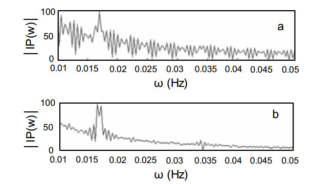
Lewis SE, DeBoer JR, Gole JL (2007) Pulsed system frequency analysis for device characterization and experimental design: Application to Porous Silicon Sensors and Extension. Sensor Actuat B-Chem 122: 20-29. doi: 10.1016/j.snb.2006.04.113
![]() |
[20] |
Laminack W, Hardy N, Baker C, et al. (2015) Approach to multi-gas sensing and modeling on nanostructure decorated porous silicon substrates. IEEE Sensors 15: 6491-6497. doi: 10.1109/JSEN.2015.2460675
![]() |
[21] | Laminack W, Baker C, Gole JL (2015) Response simulation and extraction of gas concentrations for nanostructure directed nano/microporous silicon interfaces. ECS Trans 69: 141-152. |
[22] |
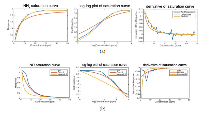
Laminack W, Gole JL (2015) Multi-gas interaction modeling on decorated semiconductor interfaces: a Fermi distribution-based isotherm and the IHSAB principle. Appl Surf Sci 359: 774-781. doi: 10.1016/j.apsusc.2015.10.110
![]() |
[23] | Laminack W, Gole JL (2016) Development of a Fermi energy distribution-based adsorption isotherm on nanostructure decorated porous substrates. ECS J Solid State Sc 5: 80-87. |
[24] |
Baker C, Laminack W, Gole JL (2016) Selective detection of inorganics NOx, SO2, and H2S in the presence of volatile BTEX contaminants toluene, benzene, and xylene. Air Qual Atmos Health 9: 411-419. doi: 10.1007/s11869-015-0350-7
![]() |
[25] |
Baker C, Ozdemir S, Gole JL (2016) Nanostructure directed detection of acidic SO2 and its transformation to basic character. J Electrochem Soc 163: B76-B82. doi: 10.1149/2.0561603jes
![]() |
[26] |
Gole JL, Goude EC, Laminack W (2012) Nanostructure driven analyte-interface electron transduction: a general approach to sensor and microreactor design. Chem Phys Chem 13: 549-561. doi: 10.1002/cphc.201100712
![]() |
[27] |
Ozdemir S, Osburn T, Gole JL (2011) A nanostructure modifiedporous silicon detection matrix for NO with demonstration of transient conversion of NO to NO2. J Electrochem Soc 158: J201-J207. doi: 10.1149/1.3583368
![]() |
[28] | Laminack W, Pouse N, Gole JL (2012) The dynamic interaction of NO2 with a nanostructure modified porous silicon matrix: the competition for donor level electrons. ECS J Solid State Sc 1: Q25-Q34. |
[29] |
Laminack W, Gole JL (2013) Nanostructure directed chemical sensing: the IHSAB principle and the effect of nitrogen and functionalization on metal oxide decorated interface response. Nanomaterials 3: 469-485. doi: 10.3390/nano3030469
![]() |
[30] |
Baker C, Laminack W, Gole JL (2015) Sensitive and selective detection of H2S and application in the presence of toluene, benzene, and xylene. Sensor Actuat B-Chem 212: 28-34. doi: 10.1016/j.snb.2015.01.123
![]() |
[31] |
Laminack W, Baker C, Gole JL (2016) Air quality and the selective detection of ammonia in the presence of toluene, benzene, and xylene. Air Qual Atmos Health 9: 231-239. doi: 10.1007/s11869-015-0329-4
![]() |
[32] | Gole JL, Ozdemir SA (2010) Nanostructure directed physisorption vs. chemisorption at semiconductor interfaces: the inverse of the hard-soft acid-base concept. ChemPhysChem 11: 2573-2581. |
[33] |
Laminack W, Baker C, Gole JL (2015) Sulphur-Hz(CHx)y(z=0,1) functionalized metal oxide nanostructure decorated interfaces: evidence of Lewis base and Bronsted acid sites- influence on chemical sensing. Mater Chem Phys 160: 20-31. doi: 10.1016/j.matchemphys.2015.03.070
![]() |
[34] |
Gole JL (2015) Increasing energy efficiency and sensitivity with simple sensor platforms. Talanta 132: 87-95. doi: 10.1016/j.talanta.2014.08.038
![]() |
[35] |
Barsan N, Schweizer-Berberich M, Göpel W (1999) Fundamental and practical aspects in the design of nanoscaled SnO2 gas sensors: a status report. Fresenius Journal of Analytical Chemistry 365: 287-304. doi: 10.1007/s002160051490
![]() |
[36] |
Comini E (2006) Metal oxide nano-crystal for gas sensing. Anal Chim Acta 568: 28-40. doi: 10.1016/j.aca.2005.10.069
![]() |
[37] |
LeGorea LJ, Lada RJ, Moulzolfa SC, et al. (2002) Defects and morphology of tungsten trioxide thin films. Thin Solid Films 406: 79-86. doi: 10.1016/S0040-6090(02)00047-0
![]() |
[38] | Rani S, Roy SC, Bhatnagar M (2006) Effects of Fe doping on the gas sensing properties of nano-crystalline SnO2 thin films. Sensor Actuat B-Chem 122: 204-210. |
[39] |
Jiménez I, Arbiol J, Dezanneau G, et al. (2003) Crystal structure, defects and gas sensor response to NO2 and H2S of tungsten trioxide nanopowders. Sensor Actuat B-Chem 93: 475-485. doi: 10.1016/S0925-4005(03)00198-9
![]() |
[40] |
Moulzolf SC, Ding S, Lad RJ (2001) Stoichiometric and microstructure effects on tungsten oxide chemirestive films. Sensor Actuat B-Chem 77: 375-382. doi: 10.1016/S0925-4005(01)00757-2
![]() |
[41] | Ponce M, Aldao C, Castro M (2003) Influence of particle size on the conductance of SnO2 thick films. J Eur Ceram Soc 23: 2105-2111. |
[42] |
Rothschild A, Komem Y (2004) The effect of grain size on the sensitivity of metal oxide gas sensors. J Appl Phys 95: 6374-6380. doi: 10.1063/1.1728314
![]() |
[43] |
Yoon DH, Choi GM (1997) Microstructure and CO gas sensing properties of porous ZnO produced by starch addition. Sensor Actuat B-Chem 45: 251-257. doi: 10.1016/S0925-4005(97)00316-X
![]() |
[44] |
Morrison SR (1987) Selectivity in semiconductor gas sensors. Sensors and Actuators 12: 425-440. doi: 10.1016/0250-6874(87)80061-6
![]() |
[45] | Watson J (1994) The stannic oxide gas sensor. Sensor Rev 14: 20-23. |
[46] | Yamazoe N, Shimiza K, Aswal DK, et al. (2007) Overview of Gas Sensor Technology. Nova Science Publishers Inc., New York. |
[47] |
Ozdemir S, Gole JL (2007) The potential of porous silicon gas sensors. Curr Opin Solid St M 11: 92-100. doi: 10.1016/j.cossms.2008.06.003
![]() |
[48] |
Lewis SE, De Boer JR, Gole JL, et al. (2005) Sensitive, selective, and analytical improvements to a porous silicon gas sensor. Sensor Actuat B-Chem 110: 54-65. doi: 10.1016/j.snb.2005.01.014
![]() |
[49] | Pearson RG (1990) Hard and soft acids and bases-the evolution of a chemical concept, Coordin Chem Rev 100: 403-425. |
[50] | Pearson RG (1997) Chemical Hardness. John Wiley VCH, Weinheim. |
[51] |
Barillaro G, Diligenti A, Nannini A, et al. (2006) Low-concentration NO2 detection with an adsorption porous silicon FET. IEEE Sens J 6: 19-23. doi: 10.1109/JSEN.2005.859360
![]() |
[52] |
Salonen J, Makila E (2018) Thermally carbonized porous silicon and recent applications. Adv Mater 30: 1703819. doi: 10.1002/adma.201703819
![]() |
[53] |
Barotta C, Faglia G, Comini E, et al. (2001) A novel porous silicon sensor for detection of sub-ppm NO2 concentrations. Sensor Actuat B-Chem 77: 62-66. doi: 10.1016/S0925-4005(01)00673-6
![]() |
[54] |
Schechter L, Ben-Chorin M, Kux A (1995) Gas sensing properties of porous silicon. Anal Chem 67: 3727-3732. doi: 10.1021/ac00116a018
![]() |
[55] |
Raghavan D, Gu X, Nguyen T, et al. (2001) Mapping chemically heterogeneous polymer system using selective chemical reaction and tapping mode atomic force microscopy. Macromolecular Symposia 167: 297-305. doi: 10.1002/1521-3900(200103)167:1<297::AID-MASY297>3.0.CO;2-2
![]() |
[56] |
Okorn-Schmidt HF (1999) Characterization of silicon surface preparation processes for advanced gate dielectrics. IBM J Res Dev 43: 351-365. doi: 10.1147/rd.433.0351
![]() |
[57] |
Boinovich LB, Elelyanenko AM (2008) Hydrophobic materials and coatings: principles of design, properities, and applications. Russ Chem Rev 77: 583-600. doi: 10.1070/RC2008v077n07ABEH003775
![]() |
[58] | Makaryan A, Sedov IV, Mozhaev PS (2016) Current state and prospects of development of technologies for the production of superhydrophobic materials and coatings. Nanotechnologies in Russia 11: 679-695. |
[59] | Ponec V, Knor Z, Cerny S (1974) Adsorption on solids. Butterworth and Co., London. |
[60] |
Gole JL, Stout J, Burda C, et al. (2004) Highly efficient formation of visible light tunable TiO2-xNx photocatalysts and their transformation at the nanoscale. J Phys Chem 108: 1230-1238. doi: 10.1021/jp030843n
![]() |
[61] |
Chen X, Lou Y, Samia ACS, et al. (2005) Formation of oxynitride as the photocatalytic enhancing site in nitrogen-doped titania nanocatalysts: comparison to a commercial nanopowder. Adv Funct Mater 15: 41-49. doi: 10.1002/adfm.200400184
![]() |
[62] |
Laminack W, Gole JL (2014) Direct in-situ nitridation of nanostructured metal oxide deposited semiconductor interfaces: tuning the response of reversibly interacting sensor sites. ChemPhysChem 15: 2473-2484. doi: 10.1002/cphc.201402108
![]() |
[63] |
Wang J, Mao B, Gole JL, et al. (2010) Visible-light-driven reversible and switchable hydrophilic to hydrophobic surfaces: correlation with photocatalysis. Nanoscale 2: 2257-2261. doi: 10.1039/c0nr00313a
![]() |
[64] |
Shi Y, He L, Guang F, et al. (2019) A review: preparation, performance, and applications of silicon oxynitride film. Micromachines 10: 552. doi: 10.3390/mi10080552
![]() |
[65] | Yount J, Lenahan P (1993) Bridging nitrogen dangling bond centers and electron trapping in amorphous NH3-nitrided and reoxidized nitride oxide films. J Non-Cryst Solids 164: 1069-1072. |
[66] |
Hori T, Naito Y, Iwasaki H, et al. (1986) Interface states and fixed charges in nanometer-range thin nitride oxides prepared by rapid thermal annealing. IEEE Electr Device L 7: 669-671. doi: 10.1109/EDL.1986.26514
![]() |
[67] |
Itakura A, Shimoda M, Kitajima M (2003) Surface stress relaxation in SiO2 by plasma nitridation and nitrogen distribution in the film. Appl Surf Sci 216: 41-45. doi: 10.1016/S0169-4332(03)00494-X
![]() |
[68] | Herzberg G (1966) Molecular Spectra and Molecular Structure. Vol. III. Electronic Spectra and Electronic Structure of Polyatomic Molecules. By O. Herzberg, D. Van Nostrand and Company, Inc.: Princeton, NJ. |
[69] |
Laminack W, Gole JL (2014) A varaiable response phosphine sensing matrix based on nanostructure treated p and n-type porous silicon interfaces. IEEE Sens J 14: 2731-2738. doi: 10.1109/JSEN.2014.2316117
![]() |
[70] | Hamilton JD (1994) Time Series Analysis. Princeton University Press, Princeton. |
[71] |
Neimark AV, Ravikovitch PI, Vishnyakov A (2000) Adsorption hysteresis in nanopores. Phys Rev E 62: R1493-1496. doi: 10.1103/PhysRevE.62.R1493
![]() |
[72] |
Barillaro G, Bruschi P, Pieri F, et al. (2007) CMOS-compatible fabrication of porous silicon gas sensors and their readout electronics on the same chip. Phys Status Solidi A 204: 1423-1428. doi: 10.1002/pssa.200674370
![]() |
[73] |
Barillaro G, Strambini LM (2008) An integrated CMOS sensing chip for NO2 detection. Sensor Actuat B-Chem 134: 585-590. doi: 10.1016/j.snb.2008.05.044
![]() |
[74] |
Baker C, Laminack W, Gole JL (2016) Modeling the absorption/desorption response of porous silicon sensors. J Appl Phys 119: 124506. doi: 10.1063/1.4944713
![]() |
1. | Masaaki Fujii, Akihiko Takahashi, Strong Convergence to the Mean Field Limit of a Finite Agent Equilibrium, 2022, 13, 1945-497X, 459, 10.1137/21M1441055 | |
2. | Masaaki Fujii, Akihiko Takahashi, Strong Convergence to the Mean-Field Limit of A Finite Agent Equilibrium, 2021, 1556-5068, 10.2139/ssrn.3905899 | |
3. | Diogo Gomes, Julian Gutierrez, Ricardo Ribeiro, A Random-Supply Mean Field Game Price Model, 2023, 14, 1945-497X, 188, 10.1137/21M1443923 | |
4. | Yuri Ashrafyan, Tigran Bakaryan, Diogo Gomes, Julian Gutierrez, 2022, The potential method for price-formation models, 978-1-6654-6761-2, 7565, 10.1109/CDC51059.2022.9992621 | |
5. | Diogo Gomes, Julian Gutierrez, Mathieu Laurière, Machine Learning Architectures for Price Formation Models, 2023, 88, 0095-4616, 10.1007/s00245-023-10002-8 | |
6. | Matt Barker, Pierre Degond, Ralf Martin, Mirabelle Muûls, A mean field game model of firm-level innovation, 2023, 33, 0218-2025, 929, 10.1142/S0218202523500203 | |
7. | Khaled Aljadhai, Majid Almarhoumi, Diogo Gomes, Melih Ucer, A mean-field game model of price formation with price-dependent agent behavior, 2024, 1982-6907, 10.1007/s40863-024-00465-0 | |
8. | Diogo Gomes, Julian Gutierrez, Mathieu Laurière, 2023, Machine Learning Architectures for Price Formation Models with Common Noise, 979-8-3503-0124-3, 4345, 10.1109/CDC49753.2023.10383244 | |
9. | Masaaki Fujii, Masashi Sekine, Mean-Field Equilibrium Price Formation With Exponential Utility, 2023, 1556-5068, 10.2139/ssrn.4420441 | |
10. | Yuri Ashrafyan, Diogo Gomes, A Fully-Discrete Semi-Lagrangian Scheme for a Price Formation MFG Model, 2025, 2153-0785, 10.1007/s13235-025-00620-y | |
11. | Masaaki Fujii, Masashi Sekine, Mean-field equilibrium price formation with exponential utility, 2024, 24, 0219-4937, 10.1142/S0219493725500017 | |
12. | Masaaki Fujii, Masashi Sekine, Mean Field Equilibrium Asset Pricing Model with Habit Formation, 2025, 1387-2834, 10.1007/s10690-024-09507-1 |