Loading [MathJax]/jax/output/SVG/jax.js
Research article Special Issues

Stoichiometric food chain model on discrete time scale

  • Stoichiometry-based models can yield many new insights into producer - grazer systems. Many interesting results can be obtained from models continuous in time. There raises the question of how robust the model predictions are to time discretization. A discrete stoichiometric food-chain model is analyzed and compared with a corresponding continuous model. Theoretical and numerical results show that the discrete and continuous models have many properties in common but differences also exist. Stoichiometric impacts of producer nutritional quality also persist in the discrete system. Both types of models can exhibit qualitatively different behaviors with the same parameter sets. Discretization enlarges the parameter ranges for the existence of chaotic dynamics. Our results suggest that the stoichiometric mechanisms are robust to time discretization and the nutritional quality of the producer can have dramatic and counterintuitive impacts on population dynamics, which agrees with the existing analysis of pelagic systems.

    Citation: Ming Chen, Meng Fan, Congbo Xie, Angela Peace, Hao Wang. Stoichiometric food chain model on discrete time scale[J]. Mathematical Biosciences and Engineering, 2019, 16(1): 101-118. doi: 10.3934/mbe.2019005

    Related Papers:

    [1] Ming Chen, Menglin Gong, Jimin Zhang, Lale Asik . Comparison of dynamic behavior between continuous- and discrete-time models of intraguild predation. Mathematical Biosciences and Engineering, 2023, 20(7): 12750-12771. doi: 10.3934/mbe.2023569
    [2] Md Nazmul Hassan, Angela Peace . Mechanistically derived Toxicant-mediated predator-prey model under Stoichiometric constraints. Mathematical Biosciences and Engineering, 2020, 17(1): 349-365. doi: 10.3934/mbe.2020019
    [3] Guangyu Sui, Meng Fan, Irakli Loladze, Yang Kuang . The dynamics of a stoichiometric plant-herbivore model and its discrete analog. Mathematical Biosciences and Engineering, 2007, 4(1): 29-46. doi: 10.3934/mbe.2007.4.29
    [4] J. David Logan, William Wolesensky, Anthony Joern . Insect development under predation risk, variable temperature, and variable food quality. Mathematical Biosciences and Engineering, 2007, 4(1): 47-65. doi: 10.3934/mbe.2007.4.47
    [5] Soumitra Pal, Pankaj Kumar Tiwari, Arvind Kumar Misra, Hao Wang . Fear effect in a three-species food chain model with generalist predator. Mathematical Biosciences and Engineering, 2024, 21(1): 1-33. doi: 10.3934/mbe.2024001
    [6] Yuanfu Shao . Bifurcations of a delayed predator-prey system with fear, refuge for prey and additional food for predator. Mathematical Biosciences and Engineering, 2023, 20(4): 7429-7452. doi: 10.3934/mbe.2023322
    [7] Maoxiang Wang, Fenglan Hu, Meng Xu, Zhipeng Qiu . Keep, break and breakout in food chains with two and three species. Mathematical Biosciences and Engineering, 2021, 18(1): 817-836. doi: 10.3934/mbe.2021043
    [8] Rajalakshmi Manoharan, Reenu Rani, Ali Moussaoui . Predator-prey dynamics with refuge, alternate food, and harvesting strategies in a patchy habitat. Mathematical Biosciences and Engineering, 2025, 22(4): 810-845. doi: 10.3934/mbe.2025029
    [9] Christian Cortés García, Jasmidt Vera Cuenca . Impact of alternative food on predator diet in a Leslie-Gower model with prey refuge and Holling Ⅱ functional response. Mathematical Biosciences and Engineering, 2023, 20(8): 13681-13703. doi: 10.3934/mbe.2023610
    [10] Christopher Middlebrook, Xiaoying Wang . A mathematical model between keystone species: Bears, salmon and vegetation. Mathematical Biosciences and Engineering, 2023, 20(9): 16628-16647. doi: 10.3934/mbe.2023740
  • Stoichiometry-based models can yield many new insights into producer - grazer systems. Many interesting results can be obtained from models continuous in time. There raises the question of how robust the model predictions are to time discretization. A discrete stoichiometric food-chain model is analyzed and compared with a corresponding continuous model. Theoretical and numerical results show that the discrete and continuous models have many properties in common but differences also exist. Stoichiometric impacts of producer nutritional quality also persist in the discrete system. Both types of models can exhibit qualitatively different behaviors with the same parameter sets. Discretization enlarges the parameter ranges for the existence of chaotic dynamics. Our results suggest that the stoichiometric mechanisms are robust to time discretization and the nutritional quality of the producer can have dramatic and counterintuitive impacts on population dynamics, which agrees with the existing analysis of pelagic systems.


    Recent advances towards the understanding of ecological interactions have been made through the development of the theory of ecological stoichiometry. Ecological stoichiometry is the study of the balance of energy (carbon) and multiple chemical elements (phosphorus, nitrogen, etc.) in ecological interactions [13]. Most ecological studies have until very recently ignored the sources and consequences of this chemical heterogeneity. The stoichiometric ratios of elements, such as carbon and phosphorus, have complex dynamics as they vary within and across trophic levels. Using the fact that all organisms are structurally composed of multiple chemical elements combined in non-arbitrary proportions, it is necessary to stress the importance of incorporating the effects of food quality, as well as quantity into ecological modeling.

    Recent efforts towards understanding predator-prey dynamics under nutritional constraints have been made with the development of stoichiometric population models [7,8,9,12,16]. Loladze et al. 2000 [8] formulated a tractable two-dimensional Lotka-Volterra type model (LKE model) that incorporates stoichiometry into the transfer of elements between producer and grazer. The LKE model provided a foundation that many stoichiometric models built upon. It utilizes the fact that both producer and grazer are chemically heterogeneous organisms. Specifically, it tracks the amount of two essential elements, C (Carbon) and P (Phosphorus), in each trophic level. Extending the LKE model to explicitly track environmental nutrient supplies, Kuang et al. 2004 [7] mechanistically formulated a tractable model of plant-herbivore population dynamics (KHE model). An additional extension of the LKE model was developed by Loladze et al. 2004, which models two competing predators on one prey (LKEF model). All these stoichiometric models show that an increase in prey quantity accompanied by decrease in its quality can halt oscillations in predator-prey system. These effects are due to the decreased energy flow from the prey to the predator. In other words, though the predator consumes more prey, it effectively converts less of it into its own biomass [5].

    It is widely recognized that the selection of time scale is very important in the study of biology and ecology [6]. The stoichiometric models mentioned above are continuous in time. This raises the question about the sensitivity of the results to the discretization of time. %After all, almost all data collected are %discrete in time. Moreover, even one dimensional discrete systems can %potentially exhibit chaos, a natural question is if the interplay between %prey quality and simple predator-prey dynamics can lead to chaos. %what effect of prey quality on the dynamics of a simple three dimensional food-chain model, especially from the point of chaos. Fan et al. [5], Sui et al. [14] and Xie et al. [17] compared the continuous stoichiometric LKE producer-grazer model [8], KHE plant-herbivore model [7] and LKEF two predators-prey model [9] to their discrete analogues, respectively. They systematically investigated the dynamic behaviors of the discrete models and conducted some comparisons with their corresponding continuous models. The results show that there are many similarities between the continuous models and their discrete analogues. However, the discrete models also exhibit new phenomenons, like chaos, not observed in the corresponding continuous models.

    Peace 2015 [11] proposed a stoichiometric model in order to investigate how stoichiometric constraints affect food-web dynamics and nutrient cycling in ecosystems. Another extension of the LKE model, this is a linear food chain with three trophic levels subject to varying carbon (light) and environmental phosphorus levels. A comprehensive global analysis of the rich dynamics (i.e., chaos) of this model is explored both analytically and numerically by Chen et al. 2017 [3]. Note that the food chain model proposed in [11] is defined on the continuous time scale, while experimental data are usually discretely collected, many producers such as annual plants have non-overlapping generations, and many herbivores have seasonal dynamics [17]. This also raises the question about the sensitivity of the main findings of this stoichiometric food chain model to the discretization of time.

    The objective of this paper is to compare the dynamics of the continuous stoichiometric tritrophic food chain model [11] with its discrete analog. In particular, we focus on these three questions: (1) whether the following most important features observed in the experiments and exhibited in the continuous stoichiometric model 'survive' the discretization, like deterministic extinction of consumers and predators when faced with low quality food; (2) whether chaotic dynamics can arise under a biologically plausible parameter set and if it does, whether the parameter ranges of the discrete model admitting chaos are the same with the continuous one; (3) whether the discrete model exhibit new mechanisms not observed by the continuous model.

    In the next three sections, we construct a discrete analogue of the stoichiometric tritrophic food chain model and explore its dynamics qualitatively. In section 5, we numerically study our discrete food chain model with Holling type Ⅱ functional response and systematically expound the similarities and differences between our discrete food chain model and its continuous analogue.

    Peace 2015 [11] proposed a three trophic level model incorporating stoichiometric principles that takes the following form:

    dxdt=bx(1xmin(K,(PTθyyθzz)/q))f(x)y,dydt=ˆeymin(1,(PTθyyθzz)/xθy)f(x)yg(y)zdyy,dzdt=ˆezmin(1,θyθz)g(y)zdzz, (2.1)

    where x is the density of producer (in milligrams of carbon per liter, mgC/L), y is the density of consumer (mgC/L), z is the density of predator (mgC/L), b is the intrinsic growth rate of producer (day1). Parameters dy and dz are the specific loss rate of consumer and predator respectively that includes metabolic losses (respiration) and death (day1). Parameters ˆey and ˆez are constant production efficiencies (yield constant) of the consumer and predator, respectively. K is the producer's constant carrying capacity that depends on some external factors such as light intensity. Functions f(x) and g(y) are the consumer's and predator's ingestion rate, which may be a Holling type Ⅱ functional responses.

    To better understand our discrete model formulation and its comparison with model (2.1), it is necessary to recall here some main assumptions of the continuous model. They are listed below:

    A1: The total mass of phosphorus in the entire system is fixed, i.e., the system is closed for phosphorus with a total of PT (mg P/L).

    A2: Producer's P (phosphorus):C (carbon) varies, but never falls below a minimum q (mg P/mg C); consumer and predator maintain a constant P:C, θy and θz (mg P/mg C), respectively.

    A3: All phosphorus in the system is divided into three pools: P in the consumer, P in the predator and P in the producer.

    Note that assumption A2 allows the producer stoichiometric P:C ratio to vary but holds the ratios higher trophic levels fixed. This strict homeostatic assumption is based on the fact that, although consumer and predator stoichiometries are variable, the range of variation is small compared to the range of producer stoichiometries. Assumption A3 does not allow for P to be dissolved in the environment, but assumes all available P for the producer is taken up immediately.

    Our discrete food chain stoichiometric model is based on the above continuous time model (2.1). There are several ways of deriving discrete time versions of dynamical systems corresponding to a continuous time formulation. Here we follow the method used in [5].

    Assume that the per capita growth rates in (2.1) change only at t=0,1,2,..., then

    1x(t)dx(t)dt=b(1x[t]min(K,(PTθyy[t]θzz[t])/q))f(x[t])y[t]x[t],1y(t)dy(t)dt=ˆeymin(1,(PTθyy[t]θzz[t])/x[t]θy)f(x[t])g(y[t])z[t]y[t]dy,1z(t)dz(t)dt=ˆezmin(1,θyθz)g(y[t])dz,t0,1,2,.... (2.2)

    Here [t] denotes the integer part of t(0,+). On any interval [n,n+1),n=0,1,2,..., we can integrate (2.2) and obtain the following equations for nt<n+1:

    x(t)=x(n)exp{[b(1x(n)min(K,(PTθyy(n)θzz(n))/q))f(x(n))y(n)x(n)](tn)},y(t)=y(n)exp{[ˆeymin(1,(PTθyy(n)θzz(n))/x(n)θy)f(x(n))g(y(n))z(n)y(n)dy](tn)},z(t)=z(n)exp{[ˆezmin(1,θyθz)g(y(n))dz](tn)}. (2.3)

    Letting tn+1, gives

    x(n+1)=x(n)exp{b(1x(n)min(K,(PTθyy(n)θzz(n))/q))f(x(n))y(n)x(n)},y(n+1)=y(n)exp{ˆeymin(1,(PTθyy(n)θzz(n))/x(n)θy)f(x(n))g(y(n))z(n)y(n)dy},z(n+1)=z(n)exp{ˆezmin(1,θyθz)g(y(n))dz}, (2.4)

    which is a discrete time analogue of (2.1). In this paper, we focus our attention on the dynamics of (2.4). Considering the biological significance of (2.4), we assume that x(0)>0, PT/θy>y(0)>0 and PT/θz>z(0)>0.

    First, we prove some preliminary results for (2.4), such as boundedness and positive invariance. It is easy to see that all components of the solution of (2.4) stay positive when they exist. By carrying out similar arguments like those in Theorem 3.1 and 3.2 in [5], we reach the following theorems.

    Table 1.  Parameters of model (2.4) with default values.
    PDescriptionValuesUnit
    PTTotal phosphorus 0.12 mg P L1
    ˆeyMaximal production efficiency in carbon terms for consumer 0.8
    ˆezMaximal production efficiency in carbon terms for predator 0.75
    bMaximal growth rate of the producer 1.2 day1
    dyConsumer loss rate (include respiration) 0.25 day1
    dzPredator loss rate (include respiration and predation) 0.003 day1
    θyConsumer constant P:C0.03 mgP/mgC
    θzPredator constant P:C0.013 mgP/mgC
    qProducer minimal P:C 0.0038mgP/mgC
    c1Maximum ingestion rate of the consumer 0.81 day1
    a1Half-saturating of consumer 0.25mg C L1
    c2Maximum ingestion rate of the predator 0.03 day1
    a2Half-saturating of predator 0.75mg C L1
    KProducer carrying capacity limited by light 010 mg C L1

     | Show Table
    DownLoad: CSV

    In Loladze [8], it is assumed that the function f(x) in system (2.4) is a bounded smooth function satisfying

    f(0)=0, f(x)>0, f(0)< and f(x)<0 for x>0.

    Also we assume the function g(y) has the same properties that

    g(0)=0, g(y)>0, g(0)< and g(y)<0 for y>0.

    In this paper, for convenience we assume that f(x)=xp(x) and g(y)=ys(y). It has been proven in [8] that

    limx0p(x)=f(0)<, p(x)<0, x>0.
    limy0s(y)=g(0)<, s(y)<0, y>0.

    Theorem 3.1. For system (2.4), we have for all n>0,

    x(n)max{x(0),Kbeb(11/b)}U,
    y(n)max{y(0),v}e2ˆeyf(U)2dyV,
    z(n)max{z(0),w}e2ˆezg(V)2dzW,

    where v and w are any numbers satisfying

    ˆeyf(ebp(U)v)<dy and ˆezg(Veˆeys(V)wdy)<dz.

    Proof. It is easy to see that the both components of the solution of equation (2.4) stay positive when exist. Notice that the function F(x)=xexpb(1x/K) achieves its maximum at x=K/b, we have

    x(n+1)<x(n)exp{bbx(n)K}Kbeb(11/b)u.

    Hence, for all nonnegative integers n, we have

    x(n)max{x(0),u}U.

    If ˆeyf(U)dy, then it is clear that for all n>0, we have y(n)y(0). We thus assume below that ˆeyf(U)>dy. Let v be large enough so that

    ˆeyf(ebp(U)v)<dy.

    We claim that for all nonnegative integers n, we have

    y(n)max{y(0),v}e2ˆeyf(U)2dyV.

    This is obviously true for n=1,2.

    Assume the above claim is false. Assume first the case that

    (Ⅰ): y(0)v. Then for some n1>2, v<y(n12)V, v<y(n11)V, and y(n1)>V. In this case, we have (using the property of p(x)<0)

    x(n11)x(n12)ebp(x(n12))y(n12)<Uebp(U)v.

    This implies that

    y(n1)<y(n11)exp{ˆeyf(Uebp(U)v)d}<y(n11)<V,

    a contradiction, indicating the claim is true for this case.

    (Ⅱ): Assume now the case of y(0)>v. In this case, we have

    x(1)<Uebp(U)v,

    which implies that

    y(2)<y(1).

    In other words, as long as y(n)>v, then y(n+2)<y(n+1). Hence there are two possibilities, either (ⅰ) for some y(n)v for some n>0; or (ⅱ) y(n)>v for all n>0. In case of (ⅱ), we have y(n) strictly decreasing for n>1 and the claim is obviously true. In case of (ⅰ), from the proof of case (Ⅰ), we see that for y(n)<V for n>n and hence the claim is also true.

    We can also use the same method to discuss the boundedness of z(n). Let w be large enough so that

    ˆezg(Veˆeys(V)wdy)<dz.

    We claim that for all nonnegative integers n, we have

    z(n)max{z(0),w}e2ˆezg(V)2dzW.

    A straightforward consequence of the above theorem is that

    Δ={(x,y,z): 0<x<Kbeb(11/b), 0<y<v, 0<z<w}

    is positively invariant. Indeed, we have

    Theorem 3.2. For (2.4), Δ is globally attractive with respect to initial values x(0), y(0) and z(0) such that x(0)>0, PT/θy>y(0)>0 and PT/θz>z(0)>0.

    Proof. It is easy to see from the model equations and the proof of the above theorem that for large values of n, x(n)(0,(K/b)eb(11/b)). Notice that if y(n)>v for large values of n>0, then y(n) must have a limit yv. Hence for large values of n, we have

    y(n)<y(n1)exp{ˆeyf(Uebp(U)v)dy}.

    Letting n yields

    yyexp{ˆeyf(Uebp(U)v)dy}<y.

    This contradicts y>v>0. Then for large values of n, y(n)(0,v). On the other side, notice that if z(n)>w for all n>0, then z(n) must have a limit zw. Hence for large values of n, we have

    z(n)<z(n1)exp{ˆezg(Veˆeys(V)wdy)dz}.

    Letting n yields

    zzexp{ˆezg(Veˆeys(V)wdy)dz}<z.

    This contradicts z>w>0, proving the theorem.

    To facilitate the equilibria analysis in the following discussion, we rewrite equation (2.4) as

    x(n+1)=x(n)exp{F(x(n),y(n),z(n))},y(n+1)=y(n)exp{G(x(n),y(n),z(n))},z(n+1)=z(n)exp{H(x(n),y(n),z(n))},

    where

    F(x,y,z)=b(1xmin(K,(PTθyyθzz)/q))p(x)y,G(x,y,z)=ˆeymin(1,(PTθyyθzz)/xθy)f(x)s(y)zdy,H(x,y,z)=ˆezmin(1,θyθz)g(y)dz.

    To find equilibria of equation (2.4) we solve

    x[1exp{F(x,y,z)}]=0, i.e., x=0 or F(x,y,z)=0,y[1exp{G(x,y,z)}]=0, i.e., y=0 or G(x,y,z)=0,z[1exp{H(x,y,z)}]=0, i.e., z=0 or H(x,y,z)=0.

    The variational matrix of equation (2.4), after some straightforward algebraic calculations, reads

    J(x,y,z)=(eF+xeFFxxeFFyxeFFzyeGGxeG+yeGGyyeGGzzeHHxzeHHyeH+zeHHz),

    where

    Fx=Fx=bmin(K,(PTθyyθzz)/q)p(x)y, (4.1)
    Fy=Fy={p(x)<0,qK+θyy+θzz<PT,bqθyx(PTθyyθzz)2p(x)<0,qK+θyy+θzz>PT. (4.2)
    Fz=Fz={0,qK+θyy+θzz<PT,bqθzx(PTθyyθzz)2<0,qK+θyy+θzz>PT. (4.3)
    Gx=Gx={ˆeyf(x)>0,θyx+θyy+θzz<PT,ˆeyPTθyyθzzθyp(x)<0,θyx+θyy+θzz>PT. (4.4)
    Gy=Gy={s(y)z>0,θyx+θyy+θzz<PT,ˆeyp(x)s(y)z,θyx+θyy+θzz>PT. (4.5)
    Gz=Gz={s(y)<0,θyx+θyy+θzz<PT,ˆeyθzθyp(x)s(y)<0,θyx+θyy+θzz>PT. (4.6)
    Hx=Hx=0, (4.7)
    Hy=Hy=ˆeymin(1,θyθz)g(y)>0, (4.8)
    Hz=Hx=0. (4.9)

    The possible equilibria or steady states of equation (2.4) solve the system of algebraic equations

    x[1exp{F(x,y,z)}]=0,
    y[1exp{G(x,y,z)}]=0,
    z[1exp{H(x,y,z)}]=0.

    It is easy to observe that the equilibria of equation (2.4) are exactly the same as those of equation (2.1).

    The only boundary equilibria are E0(0,0,0), E1(k,0,0) and E2(ˉx,ˉy,0).

    At the origin E0(0,0,0), the Jacobian matrix takes the form

    J(E0)=(eb000edy000edz).

    It is clear that the two characteristic roots edy and edz have magnitude less than 1 while the other has magnitude eb larger than 1. Consequently, the origin E0 is always unstable.

    At E1 the Jacobian is

    J(E1)=(1bkFy(k,0,0)kFz(k,0,0)0exp{G(k,0,0)}000edz),

    where

    G(k,0,0)=ˆeymin(1,PTkθy)f(k)dy.

    Then, we reach the following conclusion.

    Theorem 4.1. For equation (2.4), the origin E0 is always unstable. The boundary equilibrium E1 is locally asymptotically stable if

    0<b<2 and ˆeymin(1,PTkθy)f(k)<dy;

    it is unstable if

    b>2 or ˆeymin(1,PTkθy)f(k)>dy.

    Proof. If we let λ1, λ2 and λ3 be the characteristic roots of J(E1), then the condition

    0<b<2 and ˆeymin(1,PTkθy)f(k)<dy

    ensures that |λi|<1, i=1,2. While condition

    b>2 or ˆeymin(1,PTkθy)f(k)<dy

    implies λi>1 for some i.

    Remark 1. From [8], we know that G(x,0,0)=0 has a unique solution x1(0,PT/θy) and a unique solution x2(PT/θy,). G(k,0,0)>0 for k(x1,x2) and G(k,0,0)<0 for k[x1,x2]. For equation (2.1), if k(x1,x2) then E1 is unstable; if k[x1,x2] then E1 is stable. But for equation (2.4), the situation is quite different since E1 can be possibly stable or possibly unstable when k(x1,x2) or k[x1,x2].

    If p(x)=c1/(a1+x), then one can easily derive sufficient conditions for the stability of E0 and E1 in equation (2.4).

    The boundary equilibrium E2(ˉx,ˉy,0) indicates the extinction of predator. Thus E2 can be viewed as the internal equilibria of the degenerating simpler two-dimensional system with only one consumer on one producer. E2(ˉx,ˉy,0) can be studied in the x-y phase plane. Since both equations (2.1) and (2.4) have the same equilibria, from [5] we claim that equation (2.4) possibly has multiple E2-type boundary equilibria. In the following, we assume that E2 is such an equilibrium and discuss its local stability.

    The Jacobian at the predator-free equilibria E2(ˉx,ˉy,0) reads

    J(E2)=(Jsub(E2)J10exp{H(ˉx,ˉy,0)}),

    where

    Jsub(E2)=(1+ˉxFxˉxFyˉyGx1+ˉyGy) and J1=(ˉxFzˉyGz).

    We have the following theorem on the local asymptotical stability of the boundary equilibrium E2 by referenced [5].

    Theorem 4.2. If H(ˉx,ˉymax,0)=ˆezmin(1,θyθz)g(ˉymax)dz<0, where ˉymax=PTθyf1(dyˆey), then in region i (i.e., ˉy<PT/θyˉx), the following are true.

    If the producer's nullcline is increasing at E2 (i.e., Fx>0), then E2 is unstable.

    If the producer's nullcline is decreasing at E2 (i.e., Fx>0), and

    12ˉxˉyFyGx2<ˉxFx<ˉxˉyFyGx,

    then E2 is locally asymptotically stable.

    If the producer's nullcline is decreasing at E2 (i.e., Fx>0), and

    Fx>ˉyFyGx or ˉxFx<12ˉxˉyFyGx2

    then E2 is unstable.

    In region ii (i.e., ˉy<PT/θyˉx), the following are true.

    If the slope of the producer's nullcline at E2 is greater than the consumer's (i.e., Gx/Gy<Fx/Fy), then E2 is unstable.

    If the slope of the consumer's nullcline at E2 is greater than the producer's (i.e., Gx/Gy>Fx/Fy), and

    12ˉxˉy[FyGxFxGy]2<ˉxFx+ˉyGy<ˉxˉy[FyGxFxGy],

    then E2 is locally asymptotically stable.

    If the slope of the consumer's nullcline at E2 is greater than the producer's (i.e., Gx/Gy>Fx/Fy), and

    ˉxFx+ˉyGy<12ˉxˉy[FyGxFxGy]2, or
    ˉxFx+ˉyGy>ˉxˉy[FyGxFxGy],

    then E2 is unstable.

    If system (2.4) has an internal equilibrium E(x,y,z), then it satisfies

    F(x,y,z)=0 , G(x,y,z)=0 and H(x,y,z)=0.

    To determine the type of species interactions occurring at this equilibrium, it is convenient to examine the Jacobian matrix at E taking the following form,

    J(x,y,z,)=(1+xFxxFyxFzyGx1+yGyyGzzHxzHy1+zHz)=(100010001)+(x000y000z)(FxFyFzGxGyGzHxHyHz).

    Define

    M(x,y,z,)=(FxFyFzGxGyGzHxHyHz)

    as the ecosystem matrix of (2.4) at E. Due to the complexity of the system (2.4), we can not study the stability of positive equilibrium routinely by Routh-Hurwitz criteria, however we can conduct a qualitative analysis of the ecosystem matrix. In this matrix, the ij-th term measures the effect of the j-th species on the i-th species's per capita growth rate.

    If food quality is good the variable P:C ratio of the producer is larger than the fixed P:C ratio of the consumer, i.e., (PTθyyθzz)/x>θy, and the ecosystem matrix at E takes the following form

    (+/++/0+0),

    which means that the interaction between the consumer and the producer is of conventional (+,) type.

    If food quality is bad the variable P:C ratio of the producer is less than the fixed P:C ratio of the consumer, i.e., (PTθyyθzz)/x<θy, and the ecosystem matrix takes the form

    (+/+/0+0),

    which implies that the interaction between the consumer and the producer is changed from the traditional (+,) to (,). In other words, both the producer and the consumer compete with each other and the competition lies in two species not only internally but also interspecifically for the limited available P. Here, increasing the quantity of a producer population of bad quality will not promote the consumer's growth.

    An unusual and important property of (2.4) is that the sign of G/x changes from positive to negative as soon as the producer's P:C is less than that of the consumer's. This negative derivative means that, higher producer density reduces the growth rate of consumer. If the quality of the producer is bad, then any further increase in the producer's density deteriorates the quality of producer, which offsets the benefit provided by the higher producer density to the consumer that has already been limited by P. This effect is in sharp contrast to many conventional population dynamics models.

    In this section, we carry out systematic numerical simulations to verify and deepen our analytical findings and to compare them with those of the corresponding continuous system. In particular, we will discuss the impact of the discretization of the model (2.1).

    In the following, we assume that p(x)=c1/(a1+x) and s(y)=c2/(a2+y). We will numerically study the following food chain model with Holling type Ⅱ functional response

    x(n+1)=x(n)exp{b(1x(n)min(K,(PTθyy(n)θzz(n))/q))c1y(n)a1+x(n)},y(n+1)=y(n)exp{ˆeymin(1,(PTθyy(n)θzz(n))/x(n)θy)c1x(n)a1+x(n)c2z(n)a2+y(n)dy},z(n+1)=z(n)exp{ˆezmin(1,θyθz)c2y(n)a2+y(n)dz}, (5.1)

    and

    dxdt=bx(1xmin(K,(PTθyyθzz)/q))c1xya1+x,dydt=ˆeymin(1,(PTθyyθzz)/xθy)c1xya1+xc2yza2+ydyy,dzdt=ˆezmin(1,θyθz)c2yza2+ydzz. (5.2)

    In order to compare the dynamical behaviors of the discrete model (5.1) and continuous model (5.2), we carry out numerical simulations with the same parameters used in [3], which are listed in Table 1. These values are mainly selected from [2] and [15] and have been applied by [8] for guidance in setting parameters at biologically realistic values.

    The parameter K, indirectly represents the light intensity or energy input into the system. Bifurcation diagrams provide a clear and visual way to understand how the behavior of a dynamical system depends on a parameter. The bifurcation diagrams in Figure 1 illustrate how the dynamics of the populations in equations (5.1) and (5.2) vary with K. Numerical simulations of the time series for both models along the gradient of light levels K from 0 to 10 mgCL1 are shown in Figure 2 to assist in intuitive analysis.

    Figure 1.  The bifurcation curves versus K for the discrete model (ai, i=1,2,3) and continuous model (bi, i=1,2,3). The parameters are defined in Table 1 and the initial conditions are x=0.5 mg CL1, y=0.5 mg CL1 and z=0.5 mg CL1.
    Figure 2.  The parameters are defined in Table 1 and the initial conditions are x=0.5 mg CL1, y=0.5 mg CL1 and z=0.5 mg CL1. (ai) and (bi) denote the dynamics of the discrete model (5.1) and continuous model (5.2) with different K, respectively (i=1,2,...,7). Solid lines denote producer; Dashed lines denote consumer; Dotted lines denote predator.

    When the light intensity is low (e.g., 0<K<0.15 in Figure 1), the consumers and predators of the discrete and continuous models can not persist due to starvation. When K increases further (e.g., 0.15<K<0.5 in Figure 1), the consumer and predator of the two models persist at an stable equilibrium one after the other. Figure 2 (a1) and (b1) shows such a typical case with K=0.4. As K continues to increase, the stable equilibrium loses its stability to a limit cycle. This limit cycle starts with zero amplitude and grows as K is further increased within a reasonable interval (e.g., 0.5<K<0.7 in Figure 1). Both systems (5.1) and (5.2) exhibit the Rosenzweig's paradox enrichment. Figure 2 (a2) and (b2) show periodic oscillating dynamics when K=0.6. As K further increases, both dynamics of discrete and continuous models seem 'chaotic'. As a typical example, for K=1, the solution curves in Figure 2 (a3) and (b3) show all populations oscillate irregularly and admit chaos. After that, populations in both models all come back to regularly periodic status (e.g., Figure 2 (a4) and (b4) with K=4). As K increases from intermediate levels to high levels (e.g., 2.4<K<6.5 in Figure 1), the mean values of the oscillatory density of the producers of two models have a tendency to rise while that of the predators catch an opposite trend due to the bad quality of the producers. The amplitudes of the limit cycle solutions of both models gradually increase from zero, and then decrease to zero again. At a threshold value (e.g., K=6.5 in Figure 1), the limit cycles of the two models collapse and interior equilibrium E gains stability. All three species coexist at this equilibrium for a large enough range of K (e.g., 6.5<K<9.8 in Figure 1). Figure 2 (a5) and (b5) show case studies with K=8. Extremely high light intensity (e.g., 9.8<K<10 in Figure 1) leads to a catastrophic crash of both predator and consumer due to low food quality of the producer. Figure 2 (a6) and (b6) are case studies with K=10 where both predator and consumer perish. Due to the extinction of higher trophic levels, the primary level of the food chain (i.e., producer) in both discrete and continuous models tends towards its carrying capacity. This type of scenario is often observed as large algal blooms.

    The numerical simulations in Figure 1 and Figure 2 reveal that both the continuous model and its discrete analogue exhibit similar dynamics, but differences exist. There are some parameter sets that yield different dynamics for model (5.1) and (5.2). When K=1.13, populations of the continuous model tend to a positive stable equilibrium, while those of the discrete model show 'chaotic' behaviors (Figure 2 (a7) and (b7)). This phenomenon also contributes to the conclusion drawn by Fan et al 2005 [5] that discretization can destabilize the internal equilibria.

    There are some subtle but more important differences between the dynamics of equations (5.1) and (5.2). Both models exhibit chaos but at different parameter intervals (Figure 1). The simulations of the spectra of maximum Lyapunov exponent (MLE) of models (5.1) and (5.2) against K are shown in Figure 3. The maximum Lyapunov exponent of model (5.1) is positive when K varies within the interval K(0.9,2.4), while that of model (5.2) is positive for K(0.7,1.1). The internal equilibrium of equation (5.1) undergoes chaotic behavior later than the corresponding one of (5.2). Furthermore, the parameter range of model (5.1) admitting chaos is bigger than that of model (5.2). That is to say discretization can enlarge the parameter ranges for the existence of chaotic dynamics of the stoichiometric tritrophic models.

    Figure 3.  Spectrum of the maximum Lyapunov exponent (MLE) versus K (a) for the discrete model and (b) for continuous model. The parameters are defined in Table 1 and the initial conditions are x=0.5 mg CL1, y=0.5 mg CL1 and z=0.5 mg CL1.

    Continuous stoichiometric models can be used to study the balance of energy and multiple chemical elements between populations with overlapping generations. However, experimental data are usually collected on discrete time intervals, many plants in wild and agricultural settings have non-overlapping generations, and many herbivores have clear annual or seasonal dynamics [14]. Such scenarios call for discrete models. In this paper, a stoichiometric discrete model with three trophic levels is developed and analyzed. The model is a MacArthur-Rosenweig type food chain model under stoichiometric constraints and has rich dynamics. The possible attractors of model (2.4) include boundary equilibrium, internal equilibrium, limit cycles, or even a strange attractor (chaos) (see Figure 2). The theoretical and numerical results of our discrete model (2.4) show that they retain most of the important dynamical features exhibited by its continuous analogs (2.1). Figure 1 and Figure 3 suggest that the discrete model (2.4) admits the paradox of enrichment and also chaotic dynamics. These are typical dynamics of resource explicit population models, like stoichiometric predator-prey systems [3]. The common and notable point is that very low producer quality can drive the consumer and predator to deterministic extinction.

    Some important differences between the continuous and discrete models exist. The models predict qualitatively different dynamic behaviors for particular parameter sets (Figure 2 (a7) and (b7)). These results highlight the fact that discretization can destabilize the internal equilibria. When light levels are low or high (e.g., 0<K<0.7 or 2.4<K<10 in Figure 1), the discrete model (2.4) and the continuous model (2.1) exhibit similar dynamical behaviors. When light levels are at intermediate levels (e.g., 0.7<K<2.4 in Figure 1) different dynamics are predicted. Maximum Lyapunov exponents of models (2.1) and (2.4) in this region (Figure 3) show that the biologically plausible parameter range for chaotic dynamics of the discrete model (2.4) is larger than that of the continuous model (2.1). This supports Andersen's [2] and Fan's [5] argument on the possibility of chaos in discrete stoichiometric systems.

    In fact, the discretization can significantly impact the dynamics of system (2.1). We further compare the dynamics of the continuous model (2.1) and discrete model (2.4) by choosing the bifurcation parameter b, the producer's intrinsic growth rate. From the bifurcation diagram in Figure 4, one can easily observe that the dynamics of model (2.4) are very different from those of the corresponding continuous model for b larger than 2. Figure 4 exhibits another interesting limiting dynamics of model (2.4). Figure 4 (a1) shows the familiar periodic doubling route to chaos for the producer's density. However, the densities of consumer and predator crash and quickly reach zero shortly after the producer enters the chaos zone (Figure 4 (ai), i=2,3). This suggests that chaotic producer densities provide an important factor for the extinction of consumer and predator populations. This interesting and important biological insight is totally lost in the continuous model (2.1) (see Figure 4 (bi), i=1,2,3).

    Figure 4.  The bifurcation curves versus b, (ai) and (bi) for the discrete model and continuous model, respectively, where i=1,2,3. The parameters are defined in Table 1 and the initial conditions are x=0.5 mg CL1, y=0.5 mg CL1 and z=0.5 mg CL1.

    In summary, our analytical and numerical analysis suggest the following implications:

    ● For the most part, the continuous and the discrete stoichiometric models exhibit the same phenomena. Our discrete model retains most of the important dynamical features exhibited by its continuous analogs. Our analysis shows that qualitatively, the stoichiometric effects of food quality of producer are robust to discretization of time for particular parameter sets.

    ● Our discrete stoichiometric tritrophic model exhibits chaotic dynamics for different parameter ranges than the corresponding continuous model. Discretization enlarges the parameter ranges for the existence of chaotic dynamics.

    ● The discrete model captures some interesting results that the continuous model can not. In the discrete model, when the producer's intrinsic growth rate (b) is large, the consumer and predator can not cope with the sharp fluctuations of the producer's density and tend to perish (Figure 4). However, the continuous model predicts simplier dynamics and fails to capture this phenomenon.

    While stoichiometric effects of low food quality are presented in both continuous and discrete models, there are quantitative and qualitative effects that arise from discretization. The discretization of time illuminates the mechanism of difference between the continuous model and its discrete analog. The time scaling in ecology is very important and has crucial implications. For practical problem, it is critical that the time scale should be appropriately selected in ecology and the corresponding model can be more effective. This study can possibly serve as such an example of important insights.

    This research is partially supported by NSFC-11671072, NSFC-11271065, NSFC-11801052, RFDP-20130043110001, RFCP-CMSP-2014 and FRFCU-3132018216.

    All authors declare no conflicts of interest in this paper.


    [1] G. Ahlgren, Temperature functions in biology and their application to algal growth constants, Oikos, 49 (1987), 177–190.
    [2] T. Andersen, Pelagic nutrient cycles: herbivores as sources and sinks, Berlin: Springer, 1997.
    [3] M. Chen, M. Fan and Y. Kuang, Global dynamics in a stoichiometric food chain model with two limiting nutrients, Math. Biosci., 289 (2017), 9–19.
    [4] K. L. Edelstein, Mathematical models in biology, Siam, 1988.
    [5] M. Fan, I. Loladze, Y. Kuang and J.E.James, Dynamics of a stoichiometric discrete producergrazer model, J. Differ. Equ. Appl., 11 (2005), 347–364.
    [6] R. Frankham and B.W. Brook, The importance of time scale in conservation biology and ecology, Ann. Zool. Fenn., 41 (2004), 459–463.
    [7] Y. Kuang, J. Huisman and J. J. Elser, Stoichiometric plant-herbivore models and their interpretation, Math. Biosci. Eng., 1 (2004), 215–222.
    [8] I. Loladze, Y. Kuang and J. J. Elser, Stoichiometry in producer-grazer systems: linking energy flow with element cycling, B. Math. Biol., 62 (2000), 1137–1162.
    [9] I. Loladze, Y. Kuang, J. J. Elser and W. F. Fagan, Competition and stoichiometry: coexistence of two predators on one prey, Theor. Popul. Biol., 65 (2004), 1–15.
    [10] A. Peace, Stoichiometric Producer-Grazer Models Incorporating the Effects of Excess Food- Nutrient Content on Grazer Dynamics, Arizona State University, 2014.
    [11] A. Peace, Effects of light, nutrients, and food chain length on trophic efficiencies in simple stoichiometric aquatic food chain models, Ecol. Model., 312 (2015), 125–135.
    [12] A. Peace, H.Wang and Y. Kuang, Dynamics of a Producer-Grazer Model Incorporating the Effects of Excess Food Nutrient Content on Grazer's Growth, B. Math. Biol., 76 (2014), 2175–2197.
    [13] R. W. Sterner and J. J. Elser, Ecological stoichiometry: the biology of elements from molecules to the biosphere, Princeton University Press, 2002.
    [14] G. Sui, M. Fan, Loladze I, and Y. Kuang, The dynamics of a stoichiometric plant-herbivore model and its discrete analog, Math. Biosci. Eng., 4 (2007), 1-18.
    [15] J. Urabe and R. W. Sterner, Regulation of herbivore growth by the balance of light and nutrients, Pro. Nat. Acad. Sci., 93 (1996), 8465–8469.
    [16] H. Wang, Y. Kuang and I. Loladze, Dynamics of a mechanistically derived stoichiometric producer-grazer model, J. Biol. Dynam., 2 (2008), 286–296.
    [17] C. Xie, M. Fan andW. Zhao, Dynamics of a discrete stoichiometric two predators one prey model, J. Biol. Syst., 18 (2010), 649–667.
  • This article has been cited by:

    1. Ming Chen, Lale Asik, Angela Peace, Stoichiometric knife-edge model on discrete time scale, 2019, 2019, 1687-1847, 10.1186/s13662-019-2468-7
    2. Ling Xue, Jiayue Fu, Xinmiao Rong, Hongyu Zhang, Dynamics of a Stoichiometric Regrowth-Consumer Model, 2023, 33, 0218-1274, 10.1142/S0218127423500104
    3. Juping Ji, Russell Milne, Hao Wang, Stoichiometry and environmental change drive dynamical complexity and unpredictable switches in an intraguild predation model, 2023, 86, 0303-6812, 10.1007/s00285-023-01866-z
    4. Ming Chen, Hao Wang, Menglin Gong, Discrete-time versus continuous-time toxic predation models, 2022, 28, 1023-6198, 244, 10.1080/10236198.2022.2038586
    5. Wenting Cao, Melkamu Teshome Ayana, Rongwei Gao, Vimal Shanmuganathan, Hybrid Resource Environmental Value Chain Model Based on a Discrete Time Algorithm, 2021, 2021, 1530-8677, 1, 10.1155/2021/9993833
    6. Ming Chen, Menglin Gong, Jimin Zhang, Lale Asik, Comparison of dynamic behavior between continuous- and discrete-time models of intraguild predation, 2023, 20, 1551-0018, 12750, 10.3934/mbe.2023569
  • Reader Comments
  • © 2019 the Author(s), licensee AIMS Press. This is an open access article distributed under the terms of the Creative Commons Attribution License (http://creativecommons.org/licenses/by/4.0)
通讯作者: 陈斌, bchen63@163.com
  • 1. 

    沈阳化工大学材料科学与工程学院 沈阳 110142

  1. 本站搜索
  2. 百度学术搜索
  3. 万方数据库搜索
  4. CNKI搜索

Metrics

Article views(3881) PDF downloads(579) Cited by(6)

Figures and Tables

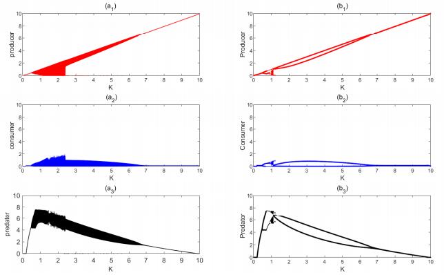
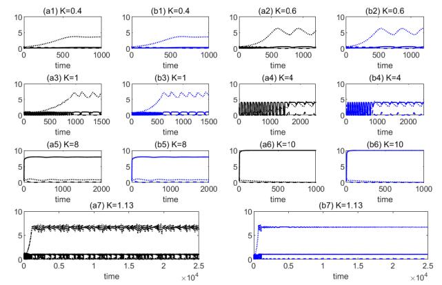
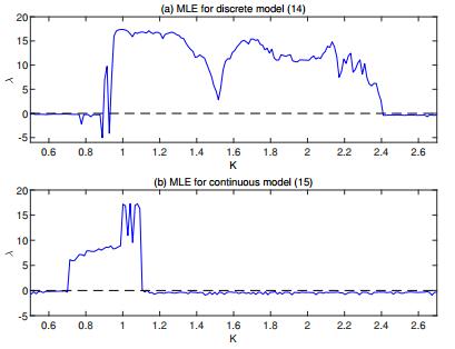
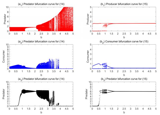
Figures(4)  /  Tables(1)

/

DownLoad:  Full-Size Img  PowerPoint
Return
Return

Catalog