Tissue-specific bioimpedance changes induced by graphene oxide <i>ex vivo</i>: a step toward contrast media development

Svetlana Kashina; Andrea Monserrat del Rayo Cervantes-Guerrero; Francisco Miguel Vargas-Luna; Gonzalo Paez; Jose Marco Balleza-Ordaz; Svetlana Kashina; Andrea Monserrat del Rayo Cervantes-Guerrero; Francisco Miguel Vargas-Luna; Gonzalo Paez; Jose Marco Balleza-Ordaz

doi:10.3934/biophy.2025005

AIMS Biophysics

2025, Volume 12, Issue 1: 54-68. doi: 10.3934/biophy.2025005

Previous Article Next Article

Research article

Tissue-specific bioimpedance changes induced by graphene oxide ex vivo: a step toward contrast media development

Svetlana Kashina ^{1
,
,},
Andrea Monserrat del Rayo Cervantes-Guerrero ¹,
Francisco Miguel Vargas-Luna ¹,
Gonzalo Paez ²,
Jose Marco Balleza-Ordaz ^{1
,
,}

1.
Division of Sciences and Engineering, University of Guanajuato. Loma del Bosque 103, Lomas del Campestre CP 37150. Leon, Guanajuato, México
2.
Center for Optics Research, Loma del Bosque 115, Colonia Lomas del Campestre León, Guanajuato, México. Código Postal 37150

Received: 22 January 2025 Revised: 25 February 2025 Accepted: 05 March 2025 Published: 11 March 2025

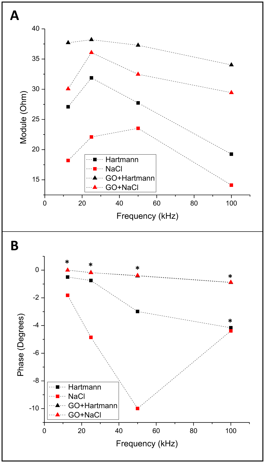
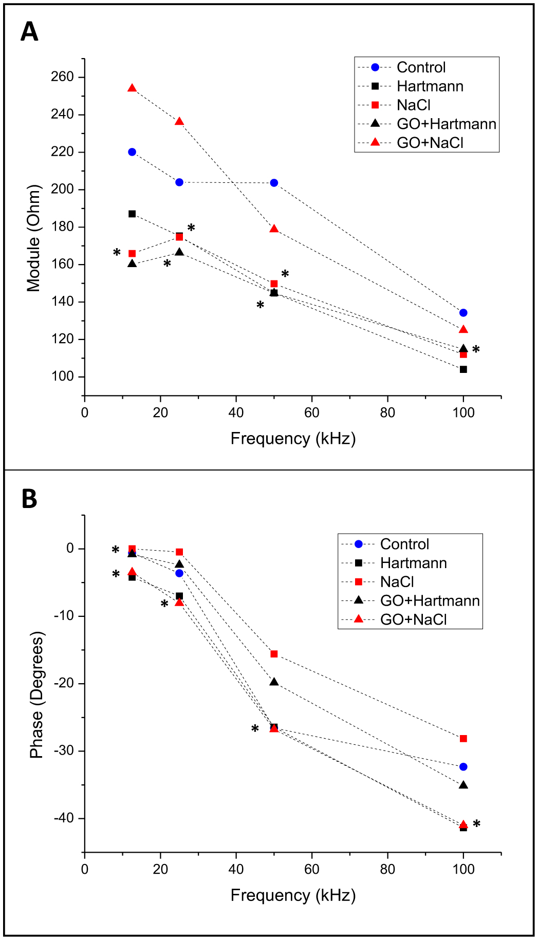
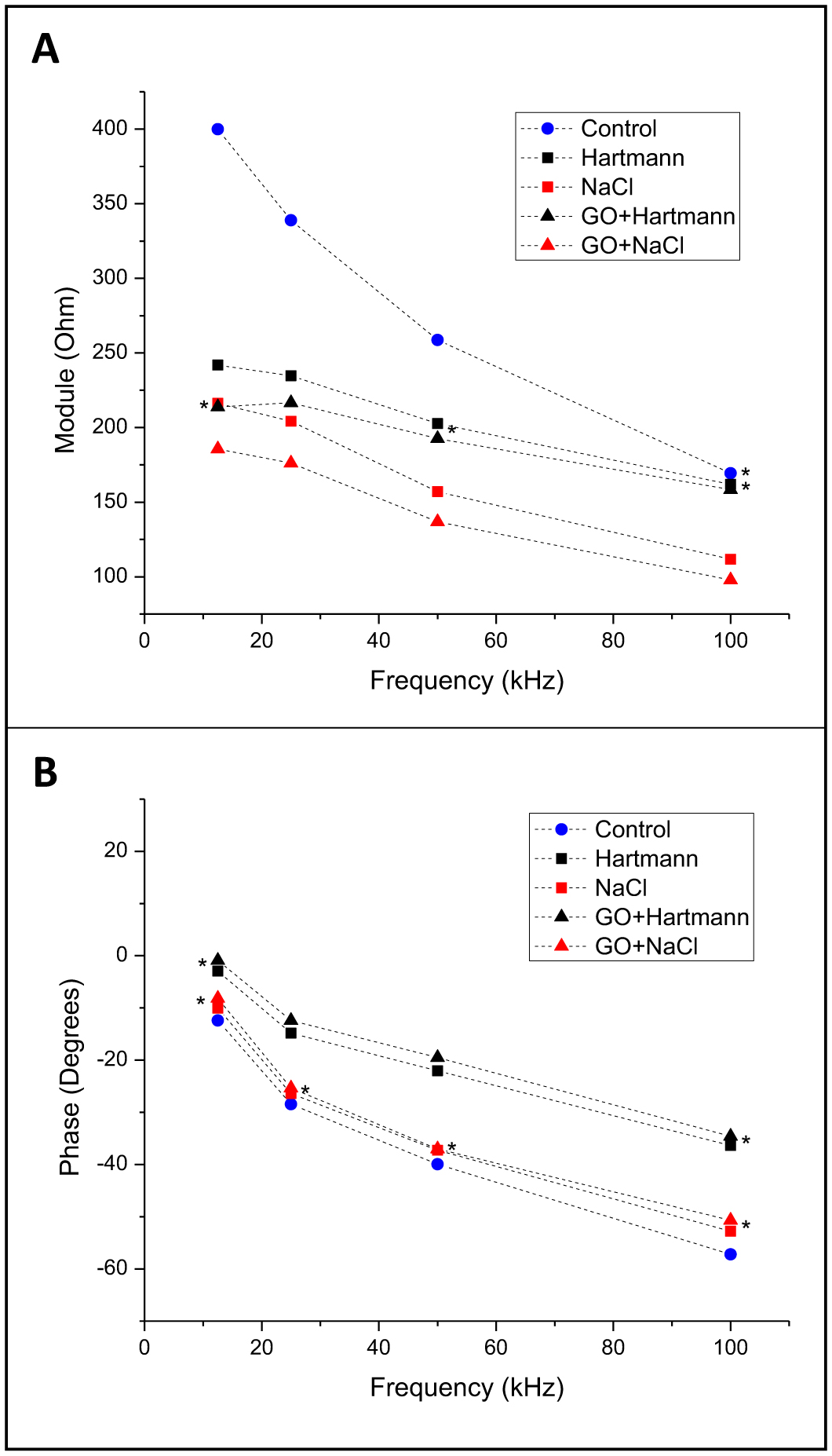
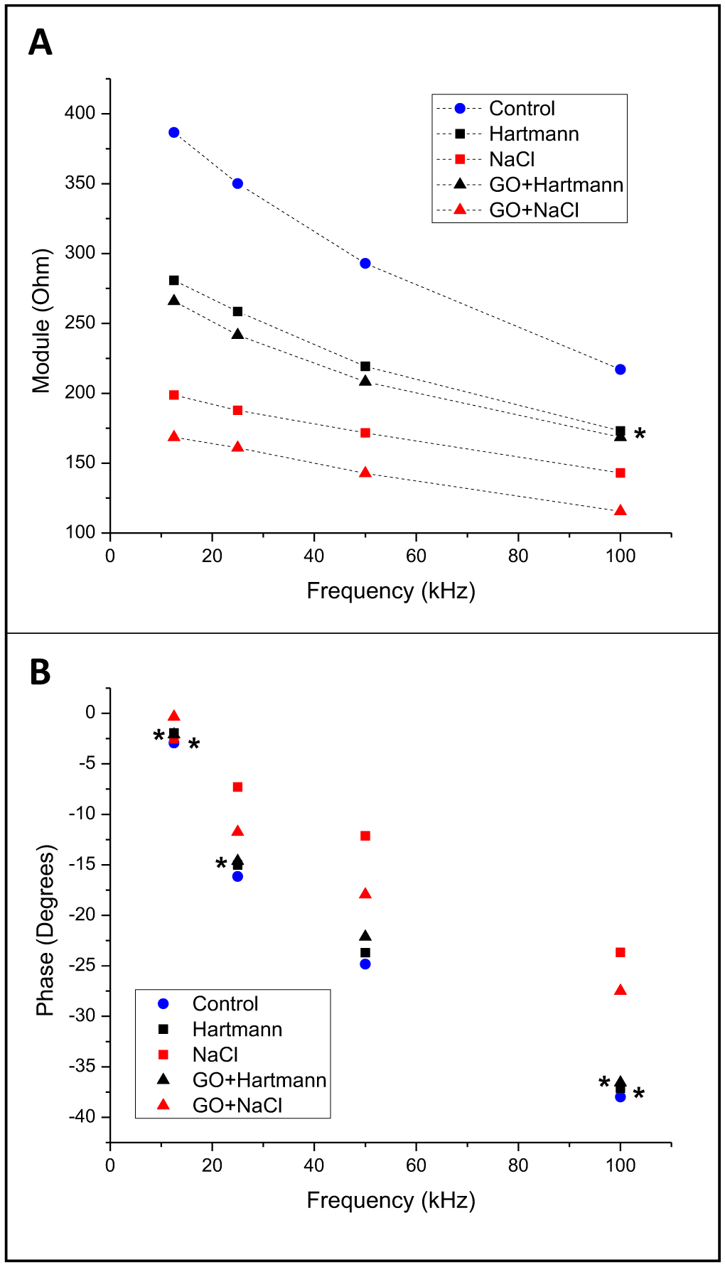
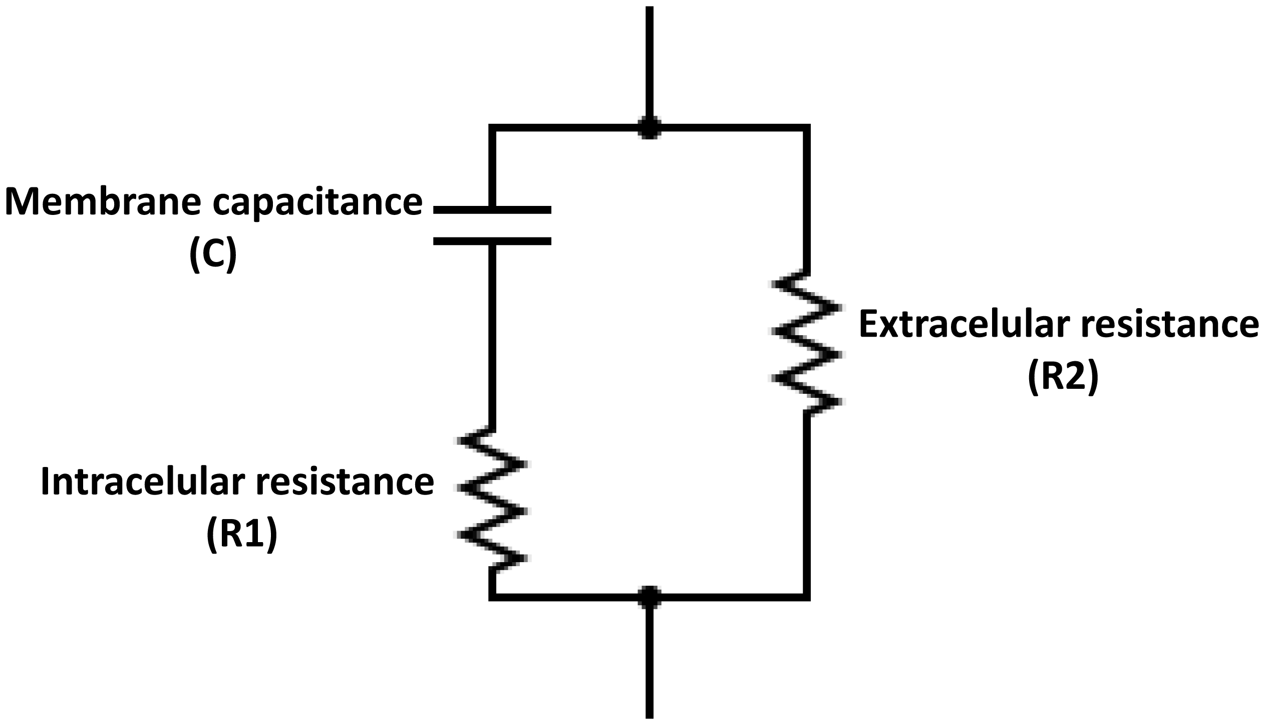
Electrical bioimpedance (BI) was proposed as an easy and cheap technique to monitor different physiological parameters. However, its clinical applications are minimal due to the low resolution and difficulties in discriminating between different tissue types. Nanoparticles have also been extensively investigated for their practical use. Graphene oxide (GO) has shown acceptable biocompatibility. The objective of this work was to assess the possibility of using GO to enhance bioimpedance measures in ex vivo models. GO was suspended in medical-grade solutions and injected into the tissues. BI was recorded at 12.5, 25, 50, and 100 kHz. Bode impedance plots evidenced statistically significant differences in tissue impedance before and after injections. Likewise, data adjustment to an equivalent electrical circuit showed that GO accumulates mainly in the extracellular space and, to some extent, at the cytoplasmatic membrane, and the accumulation is tissue specific. The latter suggests the possibility of using GO as a contrast agent to discriminate between different tissue types using BI.

Keywords:

Citation: Svetlana Kashina, Andrea Monserrat del Rayo Cervantes-Guerrero, Francisco Miguel Vargas-Luna, Gonzalo Paez, Jose Marco Balleza-Ordaz. Tissue-specific bioimpedance changes induced by graphene oxide ex vivo: a step toward contrast media development[J]. AIMS Biophysics, 2025, 12(1): 54-68. doi: 10.3934/biophy.2025005

Related Papers:

[1]	Yangrong Li, Shuang Yang, Qiangheng Zhang . Odd random attractors for stochastic non-autonomous Kuramoto-Sivashinsky equations without dissipation. Electronic Research Archive, 2020, 28(4): 1529-1544. doi: 10.3934/era.2020080
[2]	Lianbing She, Nan Liu, Xin Li, Renhai Wang . Three types of weak pullback attractors for lattice pseudo-parabolic equations driven by locally Lipschitz noise. Electronic Research Archive, 2021, 29(5): 3097-3119. doi: 10.3934/era.2021028
[3]	Shu Wang, Mengmeng Si, Rong Yang . Dynamics of stochastic 3D Brinkman-Forchheimer equations on unbounded domains. Electronic Research Archive, 2023, 31(2): 904-927. doi: 10.3934/era.2023045
[4]	Dingshi Li, Xuemin Wang . Regular random attractors for non-autonomous stochastic reaction-diffusion equations on thin domains. Electronic Research Archive, 2021, 29(2): 1969-1990. doi: 10.3934/era.2020100
[5]	Meiyu Sui, Yejuan Wang, Peter E. Kloeden . Pullback attractors for stochastic recurrent neural networks with discrete and distributed delays. Electronic Research Archive, 2021, 29(2): 2187-2221. doi: 10.3934/era.2020112
[6]	Wenlong Sun . The boundedness and upper semicontinuity of the pullback attractors for a 2D micropolar fluid flows with delay. Electronic Research Archive, 2020, 28(3): 1343-1356. doi: 10.3934/era.2020071
[7]	Xin-Guang Yang, Lu Li, Xingjie Yan, Ling Ding . The structure and stability of pullback attractors for 3D Brinkman-Forchheimer equation with delay. Electronic Research Archive, 2020, 28(4): 1395-1418. doi: 10.3934/era.2020074
[8]	Guifen Liu, Wenqiang Zhao . Regularity of Wong-Zakai approximation for non-autonomous stochastic quasi-linear parabolic equation on ${\mathbb{R}}^N$ . Electronic Research Archive, 2021, 29(6): 3655-3686. doi: 10.3934/era.2021056
[9]	Xiaojie Yang, Hui Liu, Haiyun Deng, Chengfeng Sun . Pullback $\mathcal{D}$ -attractors of the three-dimensional non-autonomous micropolar equations with damping. Electronic Research Archive, 2022, 30(1): 314-334. doi: 10.3934/era.2022017
[10]	Guowei Liu, Hao Xu, Caidi Zhao . Upper semi-continuity of pullback attractors for bipolar fluids with delay. Electronic Research Archive, 2023, 31(10): 5996-6011. doi: 10.3934/era.2023305

Abstract

1. Introduction

Meningitis is a disease of the central nervous system that leads to soreness of the lining around the brain and spinal cord. It is an acute inflammation of the defensive membranes covering the brain and spinal cord, collectively known as the meninges. This occurs when fluid surrounding the meninges is infected. Meningitis may be fatal because of the severe nature of inflammation of the brain and spinal cord, so the illness is treated as a medical emergency ^[1]. If not treated immediately, it can lead to permanent disability, coma, brain swelling, or even death. It is mainly detected by a lumbar puncture where a needle is used to extract a sample of cerebrospinal fluid from the spinal canal. It can also be diagnosed by brain imaging such as computerized tomography scan or magnetic resonance imaging, swab of fluid from the nose or throat, and blood and urine testing ^[2].

Meningitis infections can be caused by different pathogens, but most of these infections are attributed to virus, which is the least serious type with the next common cause being bacteria, fungi and parasites ^[3]. Bacterial meningitis is the most severe and epidemic-prone disease, affecting a significant part of the world's population. The bacteria are present worldwide, although in Africa, the disease is endemic to the meningitis belt. The meningitis belt spans from the Atlantic Ocean to the Red Sea, semi-arid area of sub-Saharan Africa. There is also a high tendency for outbreaks to spread across countries due to the insecure state of African borders. Other sub-Saharan African countries have also recorded large outbreaks ^[4].

Case fatality rates, which are often between 1 and 2 days after the onset of symptoms, may be as high as 50–80% when not treated and approximately 8–15% when treated ^[5]. The northern part of Ghana, namely, the Northern, North East, Savannah, Upper East and Upper West regions, lies completely in the meningitis belt and has experienced recurrent outbreaks, often during dry weather seasons characterized by low humidity, high temperatures and abundance of dust. The Brong Ahafo, Bono East and upper parts of the Volta region have also recorded sporadic cases ^[6].

Figure 1 shows the geographic distribution of meningitis in West African affected countries.

Figure 1. Areas of Africa with frequent epidemics of meningitis ^[7].

DownLoad: Full-Size Img PowerPoint

Bacterial meningitis was initially transmitted from an animal to a human being but has since become a person-to-person transmission through infected air droplets, saliva, respiratory secretions and direct contact with contaminated surfaces. The infection spreads easily when an infected person comes into close proximity or has long-term contact with others. Staying in overcrowded housing, attending sports or cultural events, sharing utensils, coughing, sneezing and kissing can all contribute to disease outbreaks ^[8].

Bacterial meningitis is caused by some strains of bacteria such as Streptococcus pneumoniae (pneumococcus), Neisseria meningitidis (meningococcus), Haemophilus influenzae (Haemophilus) and Listeria monocytogenes (Listeria). Neisseria meningitidis, Streptococcus pneumoniae and Haemophilus influenzae type B were the most common bacteria, accounting for over 80% of all bacterial meningitis cases. Meningitis caused by Haemophilus influenzae type B is much less common, now that the Haemophilus influenzae type B vaccine is administered to all children as part of routine immunization ^[1].

Most patients recover well after prompt treatment; however, several patients experience severe health complications even after prompt treatment. These complications include hearing impairments, neurological disabilities and loss of limb function ^[9]. The estimated risk of at least one complication after recovery is nearly 4 out of every 10 patients, with a median risk of approximately 20% in such patients ^[10].

The awareness of bacterial meningitis as a vaccine-preventable disease is commendable, but a number of people may not know that these vaccines are strain specific. Several previous researchers have used mathematical models to analyze the transmission and control dynamics of bacterial meningitis ^{[11,12,13,14]}. For models that consider vaccination, there is a common assumption that the vaccine does not confer immunity to all recipients, and is used as a means of treatment for infected people. However, this assumption must be lifted, as it is nowhere close to the real-life situation where the available vaccines confer varying degrees of duration of immunity against the specified strain. Furthermore, these specific vaccines are used for prevention (routine immunization) and in response to outbreaks (prompt reactive vaccination) but not for treatment ^[15].

The dynamics of cerebrospinal meningitis in the Jirapa district of the Upper West region of Ghana was presented via mathematical modeling by ^[13]. The existence of a solution to the model and its stability were examined. It was discovered that early treatment, adherance to cerebrospinal meningitis protocols, and the combined efforts of medical personnel and traditional healers could help control the disease.

In ^[16,17], an age-structured mathematical model of meningitis A (MenA) transmission, colonization and disease in the African meningitis belt was formulated and used to investigate the effects of various vaccination strategies. The validity of the model was assessed by comparing the simulated incidence of invasive MenA and the prevalence of MenA carriage with the observed incidence and carriage data. The model was able to reproduce the observed dynamics of MenA epidemics in the African meningitis belt, including seasonal increases in incidence, with large epidemics occurring every 8–12 years. It was established that the most effective modeled vaccination strategy is to conduct mass vaccination campaigns every 5 years for children aged 1–5 years.

Research ^[18] also used mathematical models to identify the crucial factors determining the dynamics of meningitis. Their simulated results suggest that temporal population immunity plays a key role and should be considered during disease monitoring and assessment of the efficiency of the vaccines deployed. A deterministic model for meningococcal meningitis transmission dynamics with variable total population size was presented in ^[19]. It was shown analytically and numerically that the disease can be eradicated using effective control measures. Their simulation suggested control measures that can reduce the disease transmission rate and immunity waning rate, as well as boost the vaccination and treatment rates.

A discrete mathematical model for the spread of meningococcal meningitis using cellular automata on graphs was presented in ^[20]. The discrete nature of the mathematical objects used in the algorithm renders model implementation simple and efficient. It was concluded that both the individual and global behaviours of the disease could be determined.

Research^[21] presented a nonlinear deterministic model on the dynamics of bacterial meningitis by incorporating time-dependent controls. Their results showed that carriers had a more significant effect on disease transmission than did the infectious class. This can be attributed to the fact that symptomatic patients are often admitted during the acute phase of the infection. This model was formulated as an optimal control problem to determine the optimal strategies for disease control. It was ascertained that vaccination played a key role in curtailing the spread of the disease. Hence, stakeholders are admonished for pushing for existing or new vaccines and antibiotics to be disbursed in the most affected areas.

To study the dynamics of the 2017 meningitis outbreak in Nigeria, ^[22] presented a deterministic model for meningitis caused by Neisseria meningitidis. This model was used to investigate the optimal strategy for curtailing the disease spread. The results indicated that combining the two control variables is the most cost-effective strategy because it averts more infections at low costs.

Because the after-effects of meningitis are not always pleasant, ^[23] presented a susceptible-vaccinated-carrier-infected-recovered-susceptible model to study the dynamics of meningitis. They distinguished between those who recovered with disabilities and those who did not. Their model suggests that a high vaccine uptake rate could control the disease. As an extension of the model for incorporating the treated population, an susceptible-vaccinated-carrier-infected-recovered deterministic compartmental model of the transmission dynamics of bacterial meningitis was presented in ^[24]. The numerical simulation results demonstrated the effects of the model parameters on each compartment, and established that efficient and effective vaccination and treatment are crucial for disease control.

Even with the availability of drugs and vaccines in the management of meningitis outbreaks, case fatality rate in Ghana remain high ranging between 36–50% ^[25]. In this study, a novel two-strain deterministic model based on the susceptible-vaccinated-carrier-infected-recovered is developed with new model parameters to obtain a more realistic model.

2. Model formulation

To formulate the model, a wide range of parameters was used to incorporate the coexistence of two bacterial meningitis strains: Streptococcus pneumoniae and Neisseria meningitidis. It is evident that the available vaccines are strain-specific ^[26], making the risk of contracting an infection from a strain one has not been vaccinated against great concern. In the proposed model, the total population at time $t$ , denoted by $N(t)$ , is divided into nine mutually exclusive epidemiological classes: the susceptible class $S(t)$ that can contract strains $1$ and $2$ , vaccinated classes $V_1(t), V_2(t)$ , carrier classes $C_1(t), C_2(t)$ , infected classes $I_1(t), I_2(t)$ , and two recovered classes $R_1(t)$ and $R_2(t)$ . Thus, $N(t)$ is given by

$\begin{align} N(t) = &S(t)+V_1(t)+V_2(t)+C_1(t)+C_2(t) \\ &+I_1(t)+I_2(t)+R_1(t)+R_2(t). \end{align}$

(2.1)

The susceptible class is a population that has not yet been infected and has not received any vaccine against the disease. This is generated by the birth or recruitment rate $\alpha$ and the loss of immunity acquired through previous vaccinations at waning rates $\omega_{1}, \omega_{2}$ . The susceptible population is reduced by infection through effective contact with infected individuals at rates $\lambda_1$ and $\lambda_2$ , which are defined as

$\begin{equation} \lambda_1 = \frac{\beta[\eta C_1(t)+I_1(t)]}{N(t)}, \end{equation}$

(2.2)

$\begin{equation} \lambda_2 = \frac{\beta[\eta C_2(t)+I_2(t)]}{N(t)}, \end{equation}$

(2.3)

where $\beta$ is the effective transmission probability per contact and $0 < \eta\leq 1$ is a modification parameter indicating the infectiousness of individuals in the carrier class. The population is also reduced by the natural death rate $\mu$ and the vaccination rates $\theta_{1}, \theta_{2}$ . Hence, the rate of change of the susceptible population is represented by the ordinary differential equation (ODE):

$\begin{equation} \frac{dS}{dt} = \alpha+\omega_1 V_1+\omega_{2} V_2-(\lambda_1+\lambda_2+\theta_1+\theta_{2}+\mu)S. \end{equation}$

(2.4)

The vaccinated class was divided into two based on the vaccines available against the two strains considered. The vaccinated population with immunity to strain 1 received pneumococcal conjugate vaccines as a form of protection against disease. This population is increased by the vaccination of susceptible individuals at rate $\theta_{1}$ . On average, pneumococcal conjugate vaccines take 2 weeks to fully kick in and should protect up to 5 years. As this vaccine does not confer immunity to all strains of bacteria causing meningitis, vaccinated individuals of strain 1 may be infected by another strain, but at a lower rate than unvaccinated individuals. This population is decreased by exposure to the disease or by vaccine waning and natural death. Therefore, the rate of change in the vaccinated population with immunity to strain 1 is represented as

$\begin{equation} \frac{dV_1}{dt} = \theta_1 S-(1-\epsilon_{1})\lambda_1V_1-(\lambda_2+\omega_1+\mu)V_1, \end{equation}$

(2.5)

where $0\leq \epsilon_{1}\leq 1$ is the level of efficacy of the pneumococcal conjugate vaccine.

The vaccinated population with immunity to strain 2 is the population of individuals who received meningococcal conjugate vaccines as a form of protection from the disease. This population is increased by vaccination of susceptible individuals to this specific strain at a rate of $\theta_{2}$ . Individuals often develop immunity within 2 weeks of receiving meningococcal conjugate vaccines and should protect them for 3–5 years. Because this vaccine does not confer immunity to all strains of bacteria causing meningitis, vaccinated individuals of strain 2 may be infected with strain 1 at an effective contact rate $\lambda_{1}$ , but at a lower rate than unvaccinated individuals. This population is decreased by exposure to infection $(1-\epsilon_{1})\lambda_{1}$ or by vaccine waning $\omega_{2}$ and natural death $\mu$ . Thus, the rate of change of the vaccinated population with immunity to strain 2 is given as

$\begin{equation} \frac{dV_2}{dt} = \theta_2 S-(1-\epsilon_{2})\lambda_2V_2-(\lambda_1+\omega_2+\mu)V_2, \end{equation}$

(2.6)

where $0\leq \epsilon_{2}\leq 1$ is the level of efficacy of the meningococcal conjugate vaccine.

The carrier population of strain 1 is made up of a population infected with Streptococcus pneumoniae but does not show any signs or symptoms even though they are infectious. This is generated by the effective contact rate $\lambda_{1}$ and decreased as a result of the population becoming symptomatic at rate $\sigma_{1}$ . This population is decreased by the recovery rate $\gamma_{C1}$ and natural death rate $\mu$ . Consequently, the rate of change in the carrier population of strain 1 is expressed as

$\begin{equation} \frac{dC_1}{dt} = \lambda_1(1-\tau_1)S+(1-\epsilon_{1})\lambda_1V_1-(\sigma_1+\gamma_{C1}+\mu)C_1, \end{equation}$

(2.7)

where $\tau_{1}$ is the proportion moving to the infected class of strain 1 without first passing through here.

The carrier population of strain 2 is composed of a population infected with Neisseria meningitidis, but do not show any signs or symptoms even though they are infectious. This is generated by the effective contact rate $\lambda_{2}$ , and decreased as a result of the progression of individuals to the infected population of strain 2 at rate $\sigma_{2}$ . This population is also decreased by the recovery rate $\gamma_{C2}$ and natural death rate $\mu$ . Therefore, the rate of change in the carrier population of strain 2 can be described by the following differential equation

$\begin{equation} \frac{dC_2}{dt} = \lambda_2(1-\tau_2)S+(1-\epsilon_{2})\lambda_2V_2-(\sigma_2+\gamma_{C2}+\mu)C_2, \end{equation}$

(2.8)

where $\tau_{2}$ is the proportion that moves to the infected class of strain 2 without first passing through the carrier population.

The infected population of strain 1 is a population with a fully blown infection of Streptococcus pneumoniae and shows signs and symptoms. This population is said to have survived an average incubation period of 1–3 days. This is also generated by the effective contact rate $\lambda_{1}$ and carrier progression at rate $\sigma_{1}$ . The population is decreased by the recovery rate $\gamma_{I1}$ , disease-induced death rate $\delta$ , and natural death rate $\mu$ . Hence, the ODE governing the dynamics of the infected population of strain 1 is given by

$\begin{equation} \frac{dI_1}{dt} = \sigma_1 C_1+\lambda_1\tau_1S+\lambda_1V_2-(\gamma_{I1}+\delta+\mu)I_1. \end{equation}$

(2.9)

The infected population of strain 2 is a population with a fully blown infection from Neisseria meningitidis that exhibits signs and symptoms of infection. This population is said to have survived an average incubation period of 4 days. This is also generated by the force of infection $\lambda_{2}$ and the progression of the carrier at the rate $\sigma_{2}$ . The population is decreased by the recovery rate $\gamma_{I2}$ , disease-induced death rate $\delta$ , and natural death rate $\mu$ . It follows that the rate of change of the infected population of strain 2 is described by the ODE, given as

$\begin{equation} \frac{dI_2}{dt} = \sigma_2 C_2+\lambda_2\tau_2S+\lambda_2V_1-(\gamma_{I2}+\delta+\mu)I_2. \end{equation}$

(2.10)

The first recovered class, $R_1(t)$ , is the population of individuals who have fully recovered from infection by either strain. This population increases because of the recovery of carriers at rates $\gamma_{C1}, \gamma_{C2}$ and infections at rates $\gamma_{I1}, \gamma_{I2}$ . They are decreased by the complication rate after a period $\wedge$ and the natural death rate $\mu$ . Thus, the rate of change of the fully recovered population is expressed as

$\begin{equation} \frac{{dR}_{1}}{dt} = \gamma_{C1}C_1+\gamma_{C2}C_2+\gamma_{I1}\rho_1 I_1+\gamma_{I2}\rho_2 I_2-(\wedge+\mu) R_{1}. \end{equation}$

(2.11)

The second recovered class, $R_2(t)$ , is the number of individuals who recovered from infection by either strain with complications owing to the sequelae of the delibitating effects among survivors, even after recovery. This population is also increased by the recovery rates of the infected populations $\gamma_{I1}, \gamma_{I2}$ , and the complication rate $\wedge$ and decrease because of the natural death rate $\mu$ . Hence, the rate of change of the recovered with complication population is described by the ODE, given by

$\begin{equation} \frac{{dR}_{2}}{dt} = \gamma_{I1}(1-\rho_1) I_1+\gamma_{I2}(1-\rho_2) I_2+\wedge R_{1}-\mu R_{2}. \end{equation}$

(2.12)

We note that all parameters are assumed to be nonnegative in an epidemiological sense.

The model parameters and model state variables are shown in Tables 1 and 2.

Table 1. Description of model parameters ^[22,23].

Parameters	Description
$\alpha$	Birth or recruitment rate into susceptible population
$\beta$	Transmission probability
$\delta$	Disease-induced death rate
$\mu$	Natural death rate
$\sigma_1$	Rate of progression from carrier of strain $1$ to infected population of strain $1$
$\sigma_{2}$	Rate of progression from carrier of strain $2$ to infected population of strain $2$
$\gamma_{C1}$	Recovery rate of carriers of strain $1$
$\gamma_{C2}$	Recovery rate of carriers of strain $2$
$\gamma_{I1}$	Recovery rate of infected with strain $1$
$\gamma_{I2}$	Recovery rate of infected with strain $2$
$\theta_1$	Strain $1$ vaccine uptake rate
$\theta_{2}$	Strain $2$ vaccine uptake rate
$\epsilon_{1}$	Strain $1$ vaccine efficacy
$\epsilon_{2}$	Strain $2$ Vaccine efficacy
$\omega_1$	Vaccine waning of strain $1$
$\omega_{2}$	Vaccine waning of strain $2$
$\tau_1$	Proportion moving to $I_1$ without first passing through $C_1$
$\tau_2$	Proportion moving to $I_2$ without first passing through $C_2$
$\wedge$	Complication rate after a period of time
$\rho_1$	Proportion moving to $R_1(t)$ from strain $1$ without first passing through $R_2(t)$
$\rho_2$	Proportion moving to $R_1(t)$ from strain $2$ without first passing through $R_2(t)$

| Show Table

DownLoad: CSV

Table 2. Description of the model state variables ^[22,23].

Variables	Description
$S(t)$	Susceptible population who can contract both strains $1$ and $2$
$V_1(t)$	Vaccinated population with immunity to strain $1$
$V_2(t)$	Vaccinated population with immunity to strain $2$
$C_1(t)$	Carrier population of strain $1$
$C_2(t)$	Carrier population of strain $2$
$I_1(t)$	Infected population of strain $1$
$I_2(t)$	Infected population of strain $2$
$R_{1}(t)$	Fully recovered population from both strains $1$ and $2$
$R_{2}(t)$	Recovered with complications from both strains $1$ and $2$

| Show Table

DownLoad: CSV

2.1. Model assumptions

$(1)$ Only two strains of bacterial meningitis were considered in this study.

$(2)$ Every individual in the studied population is susceptible to one of the two strains at a given time.

$(3)$ Individuals cannot be infected by more than one bacteria strain at the same time.

$(4)$ The vaccines are only administered to the susceptible population.

$(5)$ A vaccinated individual who loses immunity will return to the susceptible class with no vaccine protection.

$(6)$ There is permanent immunity after full recovery.

2.2. Model equations

Following the descriptions given in Eqs (2.4)–(2.12) and the flow diagram of the two-strain bacterial meningitis model presented in Figure 2, the model governing the system of nine mutually exclusive ODEs for bacterial meningitis population dynamics is expressed as

$\begin{equation} \left. \begin{array}{rrl} \frac{dS}{dt}& = &\alpha+\omega_1 V_1+\omega_{2} V_2-(\lambda_1+\lambda_2+\theta_1+\theta_{2}+\mu)S, \\ \frac{dV_1}{dt}& = &\theta_1 S-(1-\epsilon_{1})\lambda_1V_1-(\lambda_2+\omega_1+\mu)V_1, \\ \frac{dV_2}{dt}& = &\theta_2 S-(1-\epsilon_{2})\lambda_2V_2-(\lambda_1+\omega_2+\mu)V_2, \\ \frac{dC_1}{dt}& = &\lambda_1(1-\tau_1)S+(1-\epsilon_{1})\lambda_1V_1-(\sigma_1+\gamma_{C1}+\mu)C_1, \\ \frac{dC_2}{dt}& = &\lambda_2(1-\tau_2)S+(1-\epsilon_{2})\lambda_2V_2-(\sigma_2+\gamma_{C2}+\mu)C_2, \\ \frac{dI_1}{dt}& = &\sigma_1 C_1+\lambda_1\tau_1S+\lambda_1V_2-(\gamma_{I1}+\delta+\mu)I_1, \\ \frac{dI_2}{dt}& = &\sigma_2 C_2+\lambda_2\tau_2S+\lambda_2V_1-(\gamma_{I2}+\delta+\mu)I_2, \\ \frac{{dR}_{1}}{dt}& = &\gamma_{C1}C_1+\gamma_{C2}C_2+\gamma_{I1}\rho_1 I_1+\gamma_{I2}\rho_2 I_2-(\wedge+\mu) R_{1}, \\ \frac{{dR}_{2}}{dt}& = &\gamma_{I1}(1-\rho_1) I_1+\gamma_{I2}(1-\rho_2) I_2+\wedge R_{1}-\mu R_{2}, \end{array}\right. \end{equation}$

(2.13)

Figure 2. The schematic flow diagram of the transmission of two-strain bacterial meningitis.

DownLoad: Full-Size Img PowerPoint

subject to the initial conditions:

$\begin{align} S(0)& = S_0, \quad V_1(0) = V_{01}, \ V_2(0) = V_{02}, \\ C_1(0)& = C_{01}, \quad C_2(0) = C_{02}, \quad I_1(0) = I_{01}, \\ I_2(0)& = I_{02}, \quad R_1(0) = R_{01}, \quad R_2(0) = R_{02}. \end{align}$

(2.14)

3. The model analysis

3.1. Invariant region and positivity of solutions

Definition 3.1. A region within which the solutions to the model are uniformly bounded is defined as $\Omega \in \Re_+^{9}$ .

From the total population in Eq (2.1), we have

$\begin{eqnarray} \frac{dN(t)}{dt}& = &\frac{dS(t)}{dt}+\frac{dV_1(t)}{dt}+\frac{dV_2(t)}{dt}+\frac{dC_1(t)}{dt}+\frac{dC_2(t)}{dt}\\&&+\frac{dI_1(t)}{dt}+\frac{dI_2(t)}{dtx}+\frac{dR_1(t)}{dt}+\frac{dR_2(t)}{dt}. \end{eqnarray}$

(3.1)

Substituting (2.13) into (3.1) and simplifying yields

$\begin{eqnarray} \frac{dN(t)}{dt}& = &\alpha-\mu N-\delta I_1-\delta I_2, \end{eqnarray}$

(3.2)

$\begin{eqnarray} \frac{dN(t)}{dt}&\leq& \alpha-\mu N(t). \end{eqnarray}$

(3.3)

Integrating both sides of Eq (3.3), we have

$\begin{equation} -\frac{1}{\mu}\ln(\alpha-\mu N)\leq t +c, \end{equation}$

(3.4)

where $c$ is the constant of integration. Thus,

$\begin{eqnarray} \ln(\alpha-\mu N)&\geq& -(\mu t +c), \end{eqnarray}$

(3.5)

$\begin{eqnarray} (\alpha-\mu N)&\geq& ke^{-\mu t}, \end{eqnarray}$

(3.6)

where $k$ is $e^c$ .

Let $N(0) = N_0,$ this implies

$\begin{equation} (\alpha-\mu N_0)\geq k. \end{equation}$

(3.7)

From (3.6) and (3.7), we get

$\begin{eqnarray} (\alpha-\mu N)&\geq& (\alpha-\mu N_0)e^{-\mu t}, \end{eqnarray}$

(3.8)

$\begin{eqnarray} N(t)&\leq& \frac{\alpha}{\mu}-\frac{(\alpha-\mu N_0)}{\mu}e^{-\mu t}, \end{eqnarray}$

(3.9)

So,

$\begin{eqnarray} N(t)&\rightarrow &\frac{\alpha}{\mu} \ \text{as} \ \ t\rightarrow \infty, \end{eqnarray}$

(3.10)

implies $N(t)\in [0, \frac{\alpha}{\mu}].$ Therefore, the feasible set of solutions of the model equations enter and remain in the invariant region

$\begin{equation} \begin{aligned} \Omega = \{(S, V_1, V_2, C_1, C_2, I_1, I_2, R_1, R_2)\in \Re_+^{9}:N(t)\leq\frac{\alpha}{\mu}\}. \end{aligned} \end{equation}$

(3.11)

Therefore, $N(t)$ is bounded; thus, the model is mathematically and epidemiologically well-posed because region $\Omega$ is positively invariant and attractive. Hence, it is sufficient to study the dynamics of model (2.13) in $\Omega$ .

Theorem 3.1. The positivity theorem: Let

$\begin{align*} \Omega = &\{(S, V_1, V_2, C_1, C_2, I_1, I_2, R_1, R_2)\in \Re_+^{9}:S_0 > 0, \\ & V_{01} > 0, V_{02} > 0, C_{01} > 0, C_{02} > 0, I_{01} > 0, \\ &I_{02} > 0, R_{01} > 0, R_{02} > 0\}, \end{align*}$

then, the solutions $(S, V_1, V_2, C_1, C_2, I_1, I_2, R_1, R_2)$ are positive for $t\geq0$ .

Proof. Considering the first equation of the model

$\begin{eqnarray*} \frac{dS}{dt}& = &\alpha+\omega_1 V_1+\omega_{2} V_2-(\lambda_1+\lambda_2+\theta_1+\theta_{2}+\mu)S, \\ \frac{dS}{dt}&\geq&-(\lambda_1+\lambda_2+\theta_1+\theta_{2}+\mu)S, \\ \int \frac{dS}{S}&\geq&-\int (\lambda_1+\lambda_2+\theta_1+\theta_{2}+\mu)dt, \\ \ln S(t)&\geq& -f(t)+c, \end{eqnarray*}$

where

$f(t) = \int (\lambda_1+\lambda_2+\theta_1+\theta_{2}+\mu)dt$

and $c$ is the constant of integration. Hence,

$\begin{equation} S(t)\geq e^{(-f(t)+c)} = A_1e^{-f(t)}, \end{equation}$

(3.12)

where $A_1 = e^c.$ From Theorem 3.1, at $t = 0$ , $S_0 > 0$ which implies $A_1 = e^c \geq 0$ since $S(0)\geq A_1$ . Consequently,

$S(t)\geq S_0e^{-f(t)} \geq 0, \ \ \ \forall t\geq 0.$

Similarly, it can be shown that

$\begin{align} \left. \begin{array}{rrl} &&V_1(t)\geq V_{01}e^{-g(t)} \geq 0, \quad \forall t\geq 0, \\ &&V_2(t)\geq V_{02}e^{-h(t)} \geq 0, \quad \forall t\geq 0, \\ &&C_1(t)\geq C_{01}e^{-k_1t} \geq 0, \quad \forall t\geq 0, \\ &&C_2(t)\geq C_{02}e^{-k_2t} \geq 0, \quad \forall t\geq 0, \\ &&I_1(t)\geq I_{01}e^{-k_3t} \geq 0, \quad \forall t\geq 0, \\ &&I_2(t)\geq I_{02}e^{-k_4t} \geq 0, \quad \forall t\geq 0, \\ &&R_1(t)\geq R_{01}e^{-k_5t} \geq 0, \quad \forall t\geq 0, \\ &&R_2(t)\geq R_{02}e^{-\mu t} \geq 0, \quad \forall t\geq 0, \end{array}\right. \end{align}$

(3.13)

where

$g(t) = \int [(1-\epsilon_{1})\lambda_1+\lambda_2+\omega_1+\mu]dt,$

$h(t) = \int [(1-\epsilon_{2})\lambda_2+\lambda_1+\omega_2+\mu]dt,$

$k_1 = (\sigma_1+\gamma_{C1}+\mu), \ \ k_2 = (\sigma_2++\gamma_{C2}+\mu),$

$k_3 = (\gamma_{I1}+\delta+\mu), \ \ k_4 = (\gamma_{I2}+\delta+\mu), \ \ k_5 = (\wedge+\mu).$

This completes the proof of the theorem. □

3.2. Existence of equilibria

For the developed model, four equilibrium points are identified when each compartment is in steady state. These are the disease-free equilibrium (DFE), endemic equilibrium and the boundary equilibrium points.

3.2.1. The DFE point

The DFE of the model is defined as $(S^*(t), V_1^*(t), V_2^*(t), 0, 0, 0, 0, 0, 0)$ satisfying

$\begin{align*} \frac{dS(t)}{dt}& = \frac{dV_1(t)}{dt} = \frac{dV_2(t)}{dt} = \frac{dC_1(t)}{dt} = \frac{dC_2(t)}{dt}\\& = \frac{dI_1(t)}{dt} = \frac{dI_2(t)}{dt} = \frac{dR_1(t)}{dt} = \frac{dR_2(t)}{dt}\\& = 0. \end{align*}$

Equating the system of equations in (2.13) to 0 and substituting

$C_1 = C_2 = I_1 = I_2 = R_1 = R_2 = 0,$

the DFE is obtained as

$\begin{equation} \begin{aligned} E_0 = \left(\frac{(\omega_1+\mu)(\omega_{2}+\mu)\alpha}{\chi \mu}, \frac{(\omega_{2}+\mu)\theta_1\alpha}{\chi \mu}, \frac{(\omega_1+\mu)\theta_2\alpha}{\chi \mu}, 0, 0, 0, 0, 0, 0\right), \end{aligned} \end{equation}$

(3.14)

where

$\begin{equation} \chi = \left( {\mu}^{2}+\mu\, \omega_{{1}}+\mu\, \omega_{{2}}+\mu\, \theta_{{1}}+\mu\, \theta_{{2}}+\omega_{{1}}\omega_{{2}}+\omega_{{1}}\theta_{{2}}+\omega_{{2}}\theta_{{1}} \right). \end{equation}$

(3.15)

3.2.2. Endemic equilibrium point

The edemic equilibrium point of the model is defined as

$(S^*(t), V_1^*(t), V_2^*(t), C_1^*(t), C_2^*(t), I_1^*(t), I_2^*(t), R_1^*(t), R_{2}^*(t))$

satisfying

3.2.3. Boundary equilibrium points

Two boundary equilibrium points denoted by $\mathcal{E}_1$ and $\mathcal{E}_2$ are defined by

$\begin{equation} \begin{aligned} \mathcal{E}_1 = (S^*(t), V_1^*(t), V_2^*(t), C_1^*(t), 0, I_1^*(t), 0, R_1^*(t), R_{2}^*(t)), \end{aligned} \end{equation}$

(3.16)

where only strain $1$ survives, and

$\begin{equation} \begin{aligned} \mathcal{E}_2 = (S^*(t), V_1^*(t), V_2^*(t), 0, C_2^*(t), 0, I_2^*(t), R_1^*(t), R_{2}^*(t)), \end{aligned} \end{equation}$

(3.17)

where only strain $2$ survives.

Solving the system of equations for $\mathcal{E}_1$ results in

$\begin{equation} \left. \begin{array}{rrl} S^{*}& = &{\frac { \left( \lambda_1+b_7 \right) \left[ \left( 1-\epsilon_1 \right) \lambda_1+b_4 \right] \alpha}{ \left( 1 -\epsilon_1 \right) {\lambda_1}^{3}+G_2{\lambda_1}^{2}+G_1\lambda_1+\mu \chi}}, \\ V_{1}^{*}& = &{\frac {\theta_1S^*}{ \left( 1-\epsilon_1 \right) \lambda_1+b_4}}, \\ V_{2}^{*}& = &{\frac{\theta_2S^*}{\lambda_1+b_7}}, \\ C_{1}^{*}& = &{\frac {\lambda_1S^* \left[ \theta_1 \left( 1-\epsilon_1\right) + \left( 1-\tau_1 \right) \left( \left( 1-\epsilon_1 \right) \lambda_1+b_4 \right) \right] }{a_2 \left( \left( 1-\epsilon_1 \right) \lambda_1+b_4 \right) }}, \\ I_{1}^{*}& = &{\frac {\lambda_{{1}}\tau_{{1}}S^*+\sigma_{{1}}C_1^*+\lambda_1V_2^*}{a_1}}, \\ R_{1}^{*}& = &{\frac {\gamma_{{{ I1}}}\rho_1I_1^*+\gamma_{{{c1}}}C_1^*}{\wedge+\mu}}, \\ R_{2}^{*}& = &{\frac {\gamma_{{{I1}}} \left[ \left( 1-\rho_1 \right) \mu+ \wedge \right] I_1^*+\gamma_{C1}\wedge C_1^*}{\mu\, \left( \wedge+\mu \right) }}, \end{array}\right. \end{equation}$

(3.18)

where

$a_1 = \gamma_{I1}+\delta+\mu, \ a_2 = \sigma_{1}+\gamma_{C1}+\mu, \ b_{{4}} = \omega_{1}+\mu, \ b_{{7}} = \omega_{2}+\mu,$

$G_{{1}} = \left[ \chi-\omega_{{1}} \left( b_{{7}}+\theta_{{2}} \right) \right] \left( 1-\epsilon_{{1}} \right) +\mu\, b_{{4}}-\omega_{{2}} \theta_{{1}}+\chi,$

$G_2 = \left( 1-\epsilon_{{1}} \right) \left( b_{{7}}+\theta_{{1}}+\theta_{{2}}+\mu \right) +b_{{4}}.$

Substituting the state solutions in Eq (3.18) into the force of infection in Eq (2.2) yields the following cubic polynomial after some computation

$\begin{align} K_1\lambda_1^{*3}+K_2\lambda_1^{*2}+K_3\lambda_1^*+K_4 = 0, \end{align}$

(3.19)

where

$\begin{equation*} \begin{aligned} K_1 = &\left( 1-\epsilon_{{1}} \right) [ \left( 1-\tau_{{1}} \right) \left( \left( \mu+\gamma_{{{\it I1}}} \right) \sigma_{{1}}+ \left( \mu+\gamma_{{{\it c1}}} \right) a_{{1}} \right)+a_{{2}} \left( \mu+ \gamma_{{{\it I1}}} \right) \tau_{{1}}], \\ K_2 = & \left( 1-\tau_{{1}} \right) [ \left(1 -\epsilon_{{1}} \right) b_{{7} }+b_{{4}}][\sigma_{{1}} \left( \mu+\gamma_{{{\it I1}}} \right) +a_{{1} } \left( \mu+\gamma_{{{\it c1}}} \right) ] \\ &+a_{{1}}\theta_{{1}} \left( 1-\epsilon_{{1}} \right) \left( \mu+\gamma_{{{\it c1}}} \right) + \left( 1-\epsilon_{{1}} \right) \left( \mu+\gamma_{{{\it I1}}} \right) [a_{{2}} \left( \tau_{{1}}b_{{7}}\right. \\ &\left.+\theta_{{2}} \right) + \sigma_{{1}}\theta_{{1}}]-\beta\, \mu\, \left( 1-\epsilon_{{1}} \right) \left( 1-\tau_{{1}} \right) \left( \eta\, a_{{1}}+\sigma_{{1 }} \right)\\ &+a_{{2}}b_{{4}}\tau_{{1}}\left( \mu+\gamma_{{{\it I1}}} \right)-\mu\, a_{{2}} \left( 1-\epsilon_{{1}} \right) \left( \beta\, \tau_{{1}}-a_{{1}} \right) , \\ K_3 = &\, \, b_{{7}}\sigma_{{1}} \left( \mu+\gamma_{{{\it I1}}} \right)[ \left( 1-\tau_{{1}} \right) b_{{4}}+ \left( 1-\epsilon_{{1}} \right) \theta_{{1}}] \\ &+ a_{{1}} b_{{7}}[ \left(1 -\tau_{{1}} \right) b_{{4}} + \left( 1-\epsilon_{{1}}\right) \theta_{{1}} ] \left( \mu+\gamma_{{{\it c1}}} \right)\\ & +a_{{2}} \left( b_{{7}}\tau_{{1}}+\theta_{{2}} \right) [ b_{{4}} \left( \mu+\gamma_{{{\it I1}}} \right) - \mu\, \beta\, \left(1 -\epsilon_{{1}} \right)]\\ &+\mu\, a_{{1}}a_{{2}} \left(1 -\epsilon_{{1}} \right) \left( \theta_{{2}}+b_{{7}} \right) +\mu\, a_{{1}}a_{{2}} \left( \theta_{{1}}+b_{{4}} \right)\\ &-\beta\, \mu\, a_{{2}}b_{{4}}\tau_{ {1}}-\mu\, \beta\, \left( \eta\, a_{{1}}+\sigma_{{1}} \right) ( \left( 1-\tau_{{1}} \right) \left(1 -\epsilon_{{1}} \right) b_{{7} } \\ & +\left( 1-\tau_{{1}} \right) b_{{4}} + \left( 1-\epsilon_{{1}} \right) \theta_{{1}}), \\ K_4 = &-\beta\, \mu\, ( -b_{{4}}b_{{7}} \left( -1+\tau_{{1}} \right) \left( \eta\, a_{{1}}+\sigma_{{1}} \right) +b_{{7}}\theta_{{1}} \left( 1-\epsilon_{{1}} \right) \left( \eta\, a_{{1}}+\sigma_{{1}} \right)\\ & + b_{{4}} \left( b_{{7}}\tau_{{1}}+\theta_{{2}} \right) a_{{2} } ) +\mu\, a_{{1}}a_{{2}}\chi, \\ = &-\beta\, \mu\, \left( b_{{7}} \left( \eta\, a_{{1 }}+\sigma_{{1}} \right) \left( \left( 1-\tau_{{1}} \right) b_{{4}}+ \left( 1-\epsilon _{{1}} \right) \theta_{{1}} \right) +b_{{4}} \left( b_{{7}}\tau_{{1}}+\theta_{{2}} \right) a_{{2}} \right)\\ & +\mu\, a_{{1}}a_{{2}}\chi, \\ = &\left( 1-{\frac {\beta\, \left( b_{{7}} \left( \eta\, a_{{1}}+\sigma_{{1}} \right) \left( \left( 1-\tau_{{1} } \right) b_{{4}}+ \left( 1-\epsilon _{{1}} \right) \theta_{{1}} \right) +b_{{4}}( b_{{7}}\tau_{{1}}+\theta_{{2}}) a_{{2} } \right) }{a_{{1}}a_{{2}}\chi}} \right) \\ &\cdot\mu\, a_{{1}}a_{{2}}\chi \\ = &\mu a_1a_2\chi\left(1-\mathcal{R}_{01}\right), \end{aligned} \end{equation*}$

and $\mathcal{R}_{01}$ is the basic reproduction number related to strain 1 as later defined in Eq (3.29).

Solving the system of equations for $\mathcal{E}_2$ results in

$\begin{align} \left. \begin{array}{lll} &S^{*} = {\frac { \left( \lambda_2+b_4 \right) \left[ \left( 1-\epsilon_2 \right) \lambda_2+b_7 \right] \alpha}{ \left( 1 -\epsilon_2 \right) {\lambda_2}^{3}+G_4{\lambda_2}^{2}+G_3\lambda_2+\mu \chi}}, \\ &V_{1}^{*} = {\frac{\theta_1S^*}{\lambda_2+b_4}}, \\ &V_{2}^{*} = {\frac {\theta_2S^*}{ \left( 1-\epsilon_2 \right) \lambda_2+b_7}}, \\ &C_{2}^{*} = {\frac {\lambda_2S^* \left[ \theta_2 \left( 1-\epsilon_2\right) + \left( 1-\tau_2 \right) \left( \left( 1-\epsilon_2 \right) \lambda_2+b_7 \right) \right] }{a_4 \left( \left( 1-\epsilon_2 \right) \lambda_2+b_7 \right) }}, \\ &I_{2}^{*} = {\frac {\lambda_{{2}}\tau_{{2}}S^*+\sigma_{{2}}C_2^*+\lambda_2V_1^*}{a_3}}, \\ &R_{1}^{*} = {\frac {\gamma_{{{ I2}}}\rho_2I_2^*+\gamma_{{{c2}}}C_2^*}{\wedge+\mu}}, \\ &R_{2}^{*} = {\frac {\gamma_{{{I2}}} \left[ \left( 1-\rho_2 \right) \mu+ \wedge \right] I_2^*+\gamma_{C2}\wedge C_2^*}{\mu\, \left( \wedge+\mu \right) }}, \end{array}\right. \end{align}$

(3.20)

where

$a_3 = \gamma_{I2}+\delta+\mu, \ \ a_4 = \sigma_{2}+\gamma_{C2}+\mu,$

$G_{{3}} = \left[ \chi-\omega_{{2}} \left( b_{{4}}+\theta_{{1}} \right) \right] \left( 1-\epsilon_{{2}} \right) +\mu\, b_{{7}}-\omega_{{1}} \theta_{{2}}+\chi,$

$G_4 = \left( 1-\epsilon_{{2}} \right) \left( b_{{4}}+\theta_{{1}}+\theta_{{2}}+\mu \right) +b_{{7}}.$

Substituting the state solutions in Eq (3.20) into the force of infection in Eq (2.3) also yields the following cubic polynomial after some computations

$\begin{align} K_5\lambda_2^{*3}+K_6\lambda_2^{*2}+K_7\lambda_2^*+K_8 = 0, \end{align}$

(3.21)

where

$\begin{equation*} \begin{aligned} K_5 = &\left( 1-\epsilon_{{2}} \right) [ \left( 1-\tau_{{2}} \right) \left( \left( \mu+\gamma_{{{\it I2}}} \right) \sigma_{{2}}+ \left( \mu+\gamma_{{{\it c2}}} \right) a_{{3}} \right) +a_{{4}} \left( \mu+ \gamma_{{{\it I2}}} \right) \tau_{{2}}], \\ K_6 = & \left( 1-\tau_{{2}} \right) [ \left(1 -\epsilon_{{2}} \right) b_{{4} }+b_{{7}}][\sigma_{{2}} \left( \mu+\gamma_{{{\it I2}}} \right) +a_{{3} } \left( \mu+\gamma_{{{\it c2}}} \right) ]\\ & +a_{{3}}\theta_{{2}} \left( 1-\epsilon_{{2}} \right) \left( \mu+\gamma_{{{\it c2}}} \right) + \left( 1-\epsilon_{{2}} \right) \left( \mu+\gamma_{{{\it I2}}} \right) [a_{{4}} \left( \tau_{{2}}b_{{4}}+\theta_{{1}} \right) + \sigma_{{2}}\theta_{{2}}]\\ &-\beta\, \mu\, \left( 1-\epsilon_{{2}} \right) \left( 1-\tau_{{2}} \right) \left( \eta\, a_{{3}}+\sigma_{{1 }} \right)\\ &-\mu\, a_{{4}} \left( 1-\epsilon_{{2}} \right) \left( \beta\tau_{{2}}-a_{{3}} \right) +a_{{4}}b_{{7}}\tau_{{2}} \left( \mu +\gamma_{{{\it I2}}} \right), \\ K_7 = &b_{{4}}\sigma_{{2}} \left( \mu+\gamma_{{{\it I2}}} \right) \left[ \left( 1-\tau_{{2}} \right) b_{{7}}+ \left( 1-\epsilon_{{2}} \right) \theta_{{2}} \right] + a_{{3}} b_{{4}} [ \left( 1-\tau_{{2}} \right) b_{{7}} \\ & +\left( 1-\epsilon_{{2}}\right) \theta_{{2}} ] \left( \mu+\gamma_{{{\it c2}}} \right)+a_{{4}} \left( b_{{4}}\tau_{{2}}+\theta_{{1}} \right) \left[ b_{{7}} \left( \mu+\gamma_{{{\it I2}}} \right) -\mu\, \beta\, \left(1 -\epsilon_{{2}} \right) \right] \\ &+\mu\, a_{{3}}a_{{4}} \left(1 -\epsilon_{{2}} \right) \left( \theta_{{1}}+b_{{4}} \right) +\mu\, a_{{3}}a_{{4}} \left( \theta_{{2}}+b_{{7}} \right)-\beta\, \mu\, a_{{4}}b_{{7}}\tau_{ {2}}\\ &-\mu\, \beta\, \left( \eta\, a_{{3}}+\sigma_{{2}} \right) \left( \left(1 -\tau_{{2}} \right) \left(1 -\epsilon_{{2}} \right) b_{{4} }+ \left( 1-\tau_{{2}} \right) b_{{7}}+ \left( 1-\epsilon_{{2}} \right) \theta_{{2}} \right), \\ K_8 = &-\beta\, \mu\, ( -b_{{4}}b_{{7}} \left( -1+\tau_{{2}} \right) \left( \eta\, a_{{3}}+\sigma_{{2}} \right)+b_{{7}}\theta_{{2}} \left( 1-\epsilon_{{2}} \right) \left( \eta\, a_{{3}}+\sigma_{{2}} \right) \\ &+b_{{7}} \left( b_{{4}}\tau_{{2}}+\theta_{{1}} \right) a_{{4} }) +\mu\, a_{{3}}a_{{4}}\chi, \\ = &-\beta\, \mu\, ( b_{{4}} \left( \eta\, a_{{3 }}+\sigma_{{2}} \right) \left( \left( 1-\tau_{{2}} \right) b_{{7}}+ \left( 1-\epsilon _{{2}} \right) \theta_{{2}} \right)\\& + b_{{7}} \left( b_{{4}}\tau_{{2}}+\theta_{{1}} \right) a_{{4}}) +\mu\, a_{{3}}a_{{4}}\chi\\ = &\mu a_3a_4\chi\left(1-\mathcal{R}_{02}\right), \end{aligned} \end{equation*}$

and $\mathcal{R}_{02}$ is the basic reproduction number relating to strain 2 as later defined in Eq (3.30).

3.3. Stability analysis of the DFE

3.3.1. The basic reproduction number

The basic reproduction number is defined as the average number of secondary infections caused by a single infectious individual in a completely susceptible population. It helps forecast the transmission potential of a disease. According to the principle of the next generation matrix, the basic reproduction number is the spectral radius of the next generation matrix $\mathscr{F} \mathscr{V}^{-1}$ in model (2.13). Following ^[27,28], the basic reproduction number associated with model (2.13) is derived as follows

$\begin{pmatrix} \frac{dC_1}{dt}\\ \frac{dI_1}{dt}\\ \frac{dC_2}{dt}\\ \frac{dI_2}{dt} \end{pmatrix} = f_i - v_i,$

with

$\begin{equation} f_i = \begin{pmatrix} \lambda_1(1-\tau_1)S+(1-\epsilon_{1})\lambda_1V_1\\ \lambda_1\tau_1S+\lambda_1V_2\\ \lambda_2(1-\tau_2)S+(1-\epsilon_{2})\lambda_2V_2\\ \lambda_2\tau_2S+\lambda_2V_1 \end{pmatrix} \end{equation}$

(3.22)

and

$\begin{equation} v_i = \begin{pmatrix} (\sigma_1+\gamma_{C1}+\mu)C_1\\ (\gamma_{I1}+\delta+\mu)I_1 - \sigma_1C_1\\ (\sigma_2+\gamma_{C2}+\mu)C_2\\ (\gamma_{I2}+\delta+\mu)I_2 - \sigma_2C_2 \end{pmatrix}, \end{equation}$

(3.23)

where, $f_i$ is the rate of appearance of new infection(s) in compartment $i$ , $v_i$ represents the rate of transfer of individuals into compartment $i$ , with $i \in [1, 2]$ .

The Jacobian of $f_i$ at $E_{0}$ is given as

$\begin{equation} \mathscr{F} = {{{ { \begin{pmatrix} {\frac {\eta\, \beta\, b_7 \left[\theta_{1}(1-\epsilon_{1})+(1-\tau_{1})b_4\right]}{\chi}} &{\frac {\beta\, b_7 \left[\theta_{1}(1-\epsilon_{1})+(1-\tau_{1})b_4\right]}{\chi}} &0&0\\ { }{\frac {\eta\, \beta\, b_4\left(b_7\tau_{1}+\theta_{2}\right)}{\chi}} &{\frac {\beta\, b_4\left(b_7\tau_{1}+\theta_{2}\right)}{\chi}} &0&0\\ 0&0&{\frac {\eta\, \beta\, b_4 \left[\theta_{2}(1-\epsilon_{2})+(1-\tau_{2})b_7\right]}{\chi}} &{\frac {\beta\, b_4 \left[\theta_{2}(1-\epsilon_{2})+(1-\tau_{2})b_7\right]}{\chi}} \\ 0&0&{ }{\frac {\eta\, \beta\, b_7\left(b_4\tau_{2}+\theta_{1}\right)}{\chi}} &{\frac {\beta\, b_7\left(b_4\tau_{2}+\theta_{1}\right)}{\chi}} \end{pmatrix}}}}} \end{equation}$

(3.24)

and that of $v_i$ at $E_{0}$ is given as

$\begin{equation} \begin{aligned} \mathscr{V} = \begin{pmatrix} \sigma_1+\gamma_{C1}+\mu & 0&0 &0 \\ - \sigma_1 & \gamma_{I1}+\delta+\mu &0&0\\ 0&0&\sigma_2+\gamma_{C2}+\mu&0\\ 0&0&- \sigma_2 & \gamma_{I2}+\delta+\mu \end{pmatrix}\end{aligned} \end{equation}$

(3.25)

with

$\begin{equation} \begin{aligned} \mathscr{V}^{-1} = \begin{pmatrix} \frac{1}{\sigma_1+\gamma_{C1}+\mu} & 0&0&0\\ \frac{\sigma_{1}}{(\sigma_1+\gamma_{C1}+\mu)(\gamma_{I1}+\delta+\mu)} & \frac{1}{\gamma_{I1}+\delta+\mu}&0&0\\ 0&0&\frac{1}{\sigma_2+\gamma_{C2}+\mu} & 0\\ 0&0&\frac{\sigma_{2}}{(\sigma_2+\gamma_{C2}+\mu)(\gamma_{I2}+\delta+\mu)} & \frac{1}{\gamma_{I2}+\delta+\mu} \end{pmatrix}.\end{aligned} \end{equation}$

(3.26)

Thus, the next generation matrix is calculated as

$\begin{equation} \begin{aligned} & G = \mathscr{F} \mathscr{V}^{-1}\\ & = \begin{pmatrix} {\frac {\eta\, \beta\, b_7 b_1(\eta\, a_1+\sigma_{1})}{\chi\, a_1a_2}} &{\frac {\beta\, b_7 b_1}{\chi\, a_1}} &0&0\\ { }{\frac {\eta\, \beta\, b_4\left(b_7\tau_{1}+\theta_{2}\right)(\eta\, a_1+\sigma_{1})}{\chi\, a_1a_2}} &{\frac {\beta\, b_4\left(b_7\tau_{1}+\theta_{2}\right)}{\chi\, a_1}} &0&0\\ 0&0&{\frac {\beta\, b_4 b_2(\eta\, a_3+\sigma_{2})}{\chi\, a_3a_4}} &{\frac {\beta\, b_4 b_2}{\chi\, a_3}} \\ 0&0&{ }{\frac {\beta\, b_7\left(b_4\tau_{2}+\theta_{1}\right)(\eta\, a_3+\sigma_{2})}{\chi\, a_3a_4}} &{\frac {\beta\, b_7\left(b_4\tau_{2}+\theta_{1}\right)}{\chi\, a_3}} \end{pmatrix}, \end{aligned} \end{equation}$

(3.27)

where,

$b_1 = \theta_{1}(1-\epsilon_{1})+(1-\tau_{1})b_4, \ \ b_2 = \theta_{2}(1-\epsilon_{2})+(1-\tau_{2})b_7.$

The eigenvalues of the matrix G in Eq (3.27) are

$\begin{equation} \lambda^T = \begin{pmatrix} 0 \\ 0\\ {\frac {\beta\, [b_{{7}} \left( \eta\, a_{{1}}+\sigma_{{1}} \right) \left( b_{{4}} \left( 1-\tau_{{1}} \right) +\theta_{{1}} \left( 1- \epsilon_{{1}} \right) \right) +a_{{2}}b_{{4}} \left( b_{{7}}\tau_{{1 }}+\theta_{{2}} \right) ]}{a_{{1}}a_{{2}}\chi}}\\ {\frac {\beta\, [b_{{4}} \left( \eta\, a_{{3}}+\sigma_{{2}} \right) \left( b_{{7}} \left( 1-\tau_{{2}} \right) +\theta_{{2}} \left( 1- \epsilon_{{2}} \right) \right) +a_{{4}}b_{{7}} \left( b_{{4}}\tau_{{2 }}+\theta_{{1}} \right) ]}{a_{{3}}a_{{4}}\chi}} \end{pmatrix}. \end{equation}$

(3.28)

Consequently, the basic reproduction number, which is the spectral radius of G is given as $\mathcal{R}_0 = \max\{\mathcal{R}_{01}, \mathcal{R}_{02}\},$ with

$\begin{equation} \begin{aligned} \mathcal{R}_{01} = {\frac {\beta\, [b_{{7}} \left( \eta\, a_{{1}}+\sigma_{{1}} \right) \left( b_{{4}} \left( 1-\tau_{{1}} \right) +\theta_{{1}} \left( 1- \epsilon_{{1}} \right) \right) +a_{{2}}b_{{4}} \left( b_{{7}}\tau_{{1 }}+\theta_{{2}} \right) ]}{a_{{1}}a_{{2}}\chi}}, \end{aligned} \end{equation}$

(3.29)

$\begin{equation} \begin{aligned} \mathcal{R}_{02} = {\frac {\beta\, [b_{{4}} \left( \eta\, a_{{3}}+\sigma_{{2}} \right) \left( b_{{7}} \left( 1-\tau_{{2}} \right) +\theta_{{2}} \left( 1- \epsilon_{{2}} \right) \right) +a_{{4}}b_{{7}} \left( b_{{4}}\tau_{{2 }}+\theta_{{1}} \right) ]}{a_{{3}}a_{{4}}\chi}}, \end{aligned} \end{equation}$

(3.30)

representing the basic reproduction numbers related to strain $1$ and $2$ , respectively.

The expression $\mathcal{R}_{01}$ in Eq (3.29) provides the expected number of newly infected individuals that would arise as a result of introducing a single case of strain 1 into a completely susceptible population ^[29]. Similarly, $\mathcal{R}_{02}$ , given by Eq (3.30), yields the expected number of newly infected individuals that would arise if a single case of strain 2 is introduced into a completely susceptible population.

3.3.2. Local stability of the DFE

Theorem 3.2. The DFE is locally asymptotically stable if $\mathcal{R}_{0} < 1$ and unstable if $\mathcal{R}_{0} > 1$ .

Using Theorem 3.2, the result in Lemma 3.1 follows immediately based on the expressions of $\mathcal{R}_{01}, \mathcal{R}_{02}$ .

Lemma 3.1. The DFE of the two-strain bacterial meningitis model in (2.13) is locally asymptotically stable if both $\mathcal{R}_{01}, \mathcal{R}_{02} < 1$ and unstable if $\mathcal{R}_{01}, \mathcal{R}_{02} > 1$ .

Definition 3.2. The DFE of model (2.13) is said to be locally stable if each eigenvalue of the associated Jacobian matrix is negative.

Following Definition 3.2, the Jacobian matrix, $J$ evaluated at $E_0$ is given as

$\begin{equation} J = {{{ { \begin{pmatrix} -b_{3}&\omega_{1}&\omega_{2}&{-\frac{\beta\, \eta\, b_4b_7}{\chi}}&{-\frac{\beta\, \eta\, b_4b_7}{\chi}}&{-\frac{\beta\, b_4b_7}{\chi}}&{-\frac{\beta\, b_4b_7}{\chi}}&0&0\\ { }\theta_{1}&-b_4&0&{-\frac{\beta\, \eta\, \theta_{1}(1-\epsilon_{1})b_7}{\chi}}&{-\frac{\beta\, \eta\, b_7\theta_{1}}{\chi}}&{-\frac{\beta\, \theta_{1}(1-\epsilon_{1})b_7}{\chi}}&{-\frac{\beta\, b_7\theta_{1}}{\chi}}&0&0\\ \theta_{2}&0&-b_7&{-\frac{\beta\, \eta\, b_4\theta_{2}}{\chi}}&{-\frac{\beta\, \eta\, \theta_{2}(1-\epsilon_{2})b_4}{\chi}}&{-\frac{\beta\, b_4 \theta_{2}}{\chi}}&{-\frac{\beta\, \theta_{2}(1-\epsilon_{2})b_4}{\chi}}&0&0\\ 0&0&0&{ }{\frac{\beta\, \eta\, b_1 b_7}{\chi}}-a_2&0&{\frac{\beta\, b_1b_7}{\chi}}&0&0&0\\ { }0&0&0&0&{\frac{\beta\, \eta\, b_2b_4}{\chi}}-a_4&0&{\frac{\beta\, b_2b_4}{\chi}}&0&0\\ 0&0&0&{\frac{\beta\, \eta\, b_{4}b_6}{\chi}}+\sigma_{1}&0&{\frac{\beta\, b_{4}b_6}{\chi}}-a_1&0&0&0\\ { }0&0&0&0&{\frac{\beta\, \eta\, b_{7}b_5}{\chi}}+\sigma_{2}&0&{\frac{\beta\, b_{7}b_5}{\chi}}-a_3&0&0\\ 0&0&0&\gamma_{C1}&\gamma_{C2}&\gamma_{I1}\rho_{1}&\gamma_{I2}\rho_{2}&-(\wedge+\mu)&0\\ 0&0&0&0&0&\gamma_{I1}(1-\rho_{1})&\gamma_{I2}(1-\rho_{2})&\wedge&-\mu\\ \end{pmatrix}}}}} \end{equation}$

(3.31)

where

$b_3 = \theta_{1}+\theta_{2}+\mu, \ \ b_5 = b_4\tau_{2}+\theta_{1}, \ \ b_6 = b_7\tau_{1}+\theta_{2}.$

The eigenvalues of the Jacobian matrix, $J$ are

$\begin{align*} \lambda_{1, 2} = & -\frac{(a_1+a_2)\chi-\beta\, \eta\, b_1b_7-\beta\, b_4b_6\pm\sqrt{W_{1}}}{2\chi}, \\ \lambda_{3, 4} = &-\frac{(a_3+a_4)\chi -\beta\, \eta\, b_2b_4-\beta\, b_5b_7\pm\sqrt{W_{2}}}{2\chi}, \\ \lambda_{5} = &-\mu, \ \ \lambda_{6} = -(\wedge+\mu), \end{align*}$

where

$\begin{align*} W_{1} = &\beta^{2}(\eta\, b_1b_7+b_4b_6)^{2}+2\chi \beta \, \eta\, b_1b_7(a_1-a_2)\\ &-2\chi \beta\, b_4b_6(a_1-a_2)+4\chi \beta\, b_1b_7\sigma_{1}+\chi ^{2}(a_1-a_2)^{2} \end{align*}$

and

$\begin{align*} W_{2} = &\beta^{2}(\eta\, b_2b_4+b_5b_7)^{2}+2\chi \beta \, \eta\, b_2b_4(a_3-a_4)\\ &-2\chi \beta\, b_5b_7(a_3-a_4)+4\chi \beta\, b_2b_4\sigma_{2}+\chi ^{2}(a_3-a_4)^{2}. \end{align*}$

The remaining three eigenvalues of $J$ are obtained as the roots of the following polynomial

$\begin{equation} c_1\lambda^{3}+c_2\lambda^{2}+c_3\lambda+c_4 \end{equation}$

(3.32)

where

$c_{1} = 1, \\ c_{2} = b_3+b_4+b_7, \\ c_{3} = b_4b_7+b_3(b_4+b_7)-\omega_{1}\theta_{1}-\omega_{2}\theta_{2} = \chi+\mu(b_3+b_4+\omega_{2}), \\ c_{4} = b_3b_4b_7-b_4\omega_{2}\theta_{2}-b_7\omega_{1}\theta_{1} = \chi \mu$ .

Applying the Routh-Hurwitz criteria to cubic polynomial in Eq (3.32).

Because all the parameters of model (2.13) are positive, it is clear that the condition of stability is established with $c_1 > 0$ , $c_2 > 0$ , $c_3 > 0$ and $c_4 > 0$ .

3.3.3. Global asymptotic stability of the DFE

The global asymptotic stability of the model in (2.13) is investigated by following ^[29,30]. The model is denoted by

$\begin{equation} \begin{cases} \frac{dX}{dt} = F(X, Y), \\ \frac{dY}{dt} = G(X, Y), \end{cases} \end{equation}$

(3.33)

where $X = (S, V_1, V_2, R_1, R_2)$ denotes the right-hand side of the uninfected population with $C_1 = C_2 = I_1 = I_2 = 0$ and $Y = (C_1, C_2, I_1, I_2)$ denotes the right-hand side of the infected population.

Theorem 3.3. The DFE is said to be globally asymptotically stable in $\Omega$ if $\mathcal{R}_{01}, \mathcal{R}_{02} < 1$ and the following two conditions hold:

$C1:$ For $\frac{dX}{dt} = F(X, 0)$ , $E_0$ is globally asymptotically stable.

$C2:$ $G(X, Y) = J\left[G(X^*, 0)\right]Y-\hat{G}(X, Y), \\ \ \ \ \hat{G}(X, Y)\geq0, \ \ \forall\, \, (X, Y)\in\Omega,$

where

$(X^*, 0) = E_0 = \left(\frac{\alpha b_4b_7}{\mu\chi}, \frac{\alpha \theta_1 b_7}{\mu\chi}, \frac{\alpha \theta_2 b_4}{\mu\chi}, 0, 0, 0, 0, 0, 0\right),$

$J\left[G(X^*, 0)\right]$ is the Jacobian of $G(X, Y)$ obtained with respect to $(C_1, \, C_2, \, I_1, \, I_2)$ and evaluated at $(X^*, 0)$ .

Proof. C1: From the model, it follows that

$\begin{equation} F(X, 0) = \left(\begin{array}{c} \alpha+\omega_1V_1+\omega_2V_2-(\theta_1+\theta_2+\mu)S\\ \theta_1S-b_4V_1\\ \theta_2S-b_7V_2\\ -(\wedge+\mu)R_1\\ \wedge R_1-\mu R_2 \end{array}\right). \end{equation}$

(3.34)

From Eq (3.34), it is clear that

$\begin{align*} E_0& = (S, V_1, V_2, C_1, C_2, I_1, I_2, R_1, R_2)\\ & = \left(\frac{\alpha b_4b_7}{\mu\chi}, \frac{\alpha \theta_1 b_7}{\mu\chi}, \frac{\alpha \theta_2 b_4}{\mu\chi}, 0, 0, 0, 0, 0, 0\right). \end{align*}$

This can be verified using the method of integrating factors. From Eq (3.34), we have

$\begin{equation} \frac{dV_1}{dt}+b_4V_1 = \theta_1S. \end{equation}$

(3.35)

The integrating factor is given as

$e^{\int b_4dt} = e^{b_4t}.$

Multiplying Eq (3.35) through by the integrating factor yields

$\begin{align*} e^{b_4t}\left(\frac{dV_1}{dt}+b_4V_1\right) = &\left(\theta_1S\right)e^{b_4t}, \\ \int \frac{d}{dt}\left(V_1e^{b_4t}\right)dt = &\theta_1\int Se^{b_4t}dt. \end{align*}$

Let

$I = \int Se^{b_4t}dt.$

Integrating by parts, we have

$u = S \implies du = S'dt$

and

$dv = e^{b_4t}\implies v = \frac{e^{b_4t}}{b_4}.$

So,

$\begin{align*} I = &\frac{Se^{b_4t}}{b_4}-\frac{1}{b_4}\int S'e^{b_4t}dt \end{align*}$

implying that

$\begin{align*} V_1e^{b_4t} = \, \theta_1\left[\frac{Se^{b_4t}}{b_4}-\frac{1}{b_4}\int S'e^{b_4t}dt\right]. \end{align*}$

Therefore,

$\begin{align} V_1 = &\, \frac{\theta_1S}{b_4}-\frac{\theta_1}{b_4e^{b_4t}}\int S'e^{b_4t}dt. \end{align}$

(3.36)

From Eq (3.36), $V_1\to\frac{\theta_1S}{b_4}$ as $t\to \infty$ .

Similarly, we can deduce from Eq (3.34) that, $V_2\to\frac{\theta_2S}{b_7}$ as $t\to \infty$ . Furthermore, from Eq (3.34), we have

$\begin{align} \frac{dS}{dt} = \alpha+\omega_1 V_1+\omega_2 V_2-(\theta_1+\theta_2+\mu)S. \end{align}$

(3.37)

Since $V_1\to\frac{\theta_1S}{b_4}$ and $V_2\to\frac{\theta_2S}{b_7}$ , Eq (3.37) is rewritten as

$\begin{align} &\frac{dS}{dt} = \alpha+ \frac{\omega_1\theta_1S}{b_4}+ \frac{\omega_2\theta_2S}{b_7}-(\theta_1+\theta_2+\mu)S, \end{align}$

(3.38)

$\begin{align} & \frac{dS}{dt}+\frac{\mu\chi}{b_4b_7}S = \alpha. \end{align}$

(3.39)

The integrating factor of Eq (3.39) is given as

$e^{\int \frac{\mu\chi}{b_4b_7}dt} = e^{\frac{\mu\chi}{b_4b_7}t}.$

Multiplying Eq (3.39) through by the integrating factor gives

$\begin{align*} e^{\frac{\mu\chi}{b_4b_7}t}\left(\frac{dS}{dt}+\frac{\mu\chi}{b_4b_7}S\right) = &\alpha e^{\frac{\mu\chi}{b_4b_7}t}, \\ \int \frac{d}{dt}\left(Se^{\frac{\mu\chi}{b_4b_7}t}\right)dt = &\int \alpha e^{\frac{\mu\chi}{b_4b_7}t}dt, \\ Se^{\frac{\mu\chi}{b_4b_7}t} = &\frac{\alpha b_4b_7}{\mu\chi} e^{\frac{\mu\chi}{b_4b_7}t}+c, \end{align*}$

where $c$ is the constant of integration. Therefore,

$\begin{align} S = \frac{\alpha b_4b_7}{\mu\chi}+Ce^{-\frac{\mu\chi}{b_4b_7}t}. \end{align}$

(3.40)

From Eq (3.40), $S\to\frac{\alpha b_4b_7}{\mu\chi}$ as $t\to\infty$ ; and this implies the global convergence of Eq (3.34) in $\Omega$ .

C2: $G(X, Y)$ is given as

$\begin{equation} G(X, Y) = \left[\begin{array}{c} \lambda_1(1-\tau_1)S+(1-\epsilon_1)\lambda_1V_1-a_2C_1\\ { }\lambda_2(1-\tau_2)S+(1-\epsilon_2)\lambda_2V_2-a_4C_2\\ { }\sigma_1C_1+\lambda_1\tau_1S+\lambda_1V_2-a_1I_1\\ { }\sigma_2C_2+\lambda_2\tau_2S+\lambda_2V_1-a_3I_2 \end{array} \right], \end{equation}$

(3.41)

where $\lambda_1$ and $\lambda_2$ are the forces of infection defined in Eqs (2.2) and (2.3).

By the condition in C2 with Eqs (3.41) and (3.43), $\hat{G}(X, Y)$ is given by

$\begin{equation} \begin{aligned} \left(\begin{array}{c} \frac{ \beta\left(\eta C_1+I_1\right)\left[\left(1-\epsilon_1\right)V_1^*+(1-\tau_1)S^*\right]}{N^*}\left(1-\frac{(1-\epsilon_1)V_1+(1-\tau_1)S}{N}\frac{N^*}{\left(1-\epsilon_1\right)V_1^*+(1-\tau_1)S^*}\right)\\ { }\frac{ \beta\left(\eta C_2+I_2\right)\left[\left(1-\epsilon_2\right)V_2^*+(1-\tau_2)S^*\right]}{N^*}\left(1-\frac{(1-\epsilon_2)V_2+(1-\tau_2)S}{N}\frac{N^*}{\left(1-\epsilon_2\right)V_2^*+(1-\tau_2)S^*}\right)\\ { }\frac{\beta\left(\eta C_1+I_1\right)\left(\tau_1S^*+V_2^*\right)}{N^*}\left(1-\frac{(\tau_1S+V_2)}{N}\frac{N^*}{(\tau_1S^*+V_2^*)}\right)\\ { }\frac{\beta\left(\eta C_2+I_2\right)\left(\tau_2S^*+V_1^*\right)}{N^*}\left(1-\frac{(\tau_2S+V_1)}{N}\frac{N^*}{(\tau_2S^*+V_1^*)}\right) \end{array} \right).\end{aligned} \end{equation}$

(3.42)

The Jacobian matrix of $G(X, Y)$ , $J\left[G(X^*, 0)\right]$ is given as

$\begin{equation} \begin{aligned} \left( \begin{array}{cccc} {\frac {\beta\, \eta\, \left[ \left( 1- \epsilon_{{1}} \right) V_1^*+ \left( 1-\tau_{{1}} \right) S^* \right] -a_{{2}}N^*}{N^*}}&0&{\frac {\beta\, \left[ \left( 1-\epsilon_{{ 1}} \right) V_1^*+ \left( 1-\tau_{{1}} \right) S^* \right] }{N^*}}&0 \\ { }0&{\frac {\beta\, \eta\, \left[ \left( 1-\epsilon _{{2}} \right) V_2^*+ \left( 1-\tau_{{2}} \right) S^* \right] -a_{{4} }N^*}{N^*}}&0&{\frac {\beta\, \left[ \left( 1-\epsilon_{{2}} \right) V_2^*+ \left( 1-\tau_{{2}} \right) S^* \right] }{N^*}} \\ { }{\frac {\beta\, \eta\, \left( \tau_{{1}}S^*+V_2^* \right) +\sigma_{{1}}N^*}{N^*}}&0&{\frac {\beta\, \left( \tau_{{1}}S^*+V_2^* \right) -a_{{1}}N^*}{N^*}}&0\\ { }0&{\frac {\beta\, \eta\, \left(\tau_{{2}}S^*+V_1^* \right) +\sigma_{{2}}N^*}{N^*}}&0&{ \frac {\beta\, \left( \tau_{{2}}S^*+V_1^*\right) -a_{{3}}N^*}{N^*}} \end{array} \right).\end{aligned} \end{equation}$

(3.43)

Since

$S^* = \frac{\alpha b_4b_7}{\mu\chi}, \, \ \ \ \ V_1^* = \frac{\alpha\theta_1b_7}{\mu\chi}, \, \ \ \ \ V_2^* = \frac{\alpha\theta_2b_4}{\mu\chi} \ \ \text{and} \ \ N^* = \frac{\alpha}{\mu},$

we have that $S\leq S^*, \, \ V_1\leq V_1^* \, \text{and} \ V_2\leq V_2^*$ . Thus, it follows that $S\leq N, \, \ V_1\leq N \, \text{and} \ V_2\leq N$ in $\Omega$ . Therefore, if the total population is at the equilibrium level, we have

$\left(1-\frac{(1-\epsilon_1)V_1+(1-\tau_1)S}{N}\frac{N^*}{\left(1-\epsilon_1\right)V_1^*+(1-\tau_1)S^*}\right) > 0,$

$\left(1-\frac{(1-\epsilon_2)V_2+(1-\tau_2)S}{N}\frac{N^*}{\left(1-\epsilon_2\right)V_2^*+(1-\tau_2)S^*}\right) > 0,$

$\left(1-\frac{(\tau_1S+V_2)}{N}\frac{N^*}{(\tau_1S^*+V_2^*)}\right) > 0$

and

$\left(1-\frac{(\tau_2S+V_1)}{N}\frac{N^*}{(\tau_2S^*+V_1^*)}\right) > 0;$

thus, $\hat{G}(X, Y)\geq0$ . Hence, it follows from Theorem 3.3 that the DFE, $E_0 = (X^*, 0)$ is globally asymptotically stable.□

3.4. Model parameter estimation and initial conditions

3.4.1. Initial conditions

The base year used in the simulations is 2017. As the disease is endemic to the northern part of Ghana, the total population of the northern part as of 2017, was 4953293 ^[31]; thus, the initial total population, $N(0) = 4953293$ . Since the outbreak that year was due to the Neisseria meningitidis strain, the initially infected individuals of strain $2$ were considered, $I_2(0) = 69$ , which is the same number reported in data. We assumed $I_1(0) = 153$ . According to a literature review, Streptococcus pneumoniae is found in the nose and throat of $20$ – $40\%$ of people, whereas Neisseria meningitidis is found in $1$ – $10\%$ of these people without causing any symptoms of illness. Thus, taking $140\%$ and $110\%$ of $I_1(0)$ and $I_2(0)$ , respectively gives $C_1(0) = 214$ and $C_2(0) = 76$ . We assumed

$V_1(0) = V_2(0) = R_1(0) = R_2(0) = 0,$

so the initial susceptible is

$S(0) = N(0)-V_1(0)-V_2(0)-C_1(0)-C_2(0)$

$-I_1(0)-I_2(0)-R_1(0)-R_2(0)$

$= 4952781.\qquad\qquad\qquad\qquad\quad\$

3.4.2. Parameter values

$(1)$ Natural death rate ( $\mu$ ): The average lifespan in Ghana is $64.17$ years. Therefore,

$\mu = \frac{1}{64.17 \times 365} = 4.269\times 10^{-5}$

per day.

$(2)$ Birth or recruitment rate ( $\alpha$ ): The limiting total human population in the absence of the disease is assumed to be $\frac{\alpha}{\mu} = 4953293$ , so $\alpha = 211$ per day.

$(3)$ Disease-induced death rate ( $\delta$ ): The mortality rate due to bacterial meningitis disease in Ghana is $36$ – $50\%$ . By taking the average of $43\%$ , we obtain that $\delta = 0.43$ .

$(4)$ Progression rates ( $\sigma_{1}, \sigma_{2}$ ): The average incubation period for Streptococcus pneumonaie is 1–3 days while Neisseria meningitidis is 4 days. Thus,

$\sigma_{1} = \frac{1}{2} = 0.5\; \; \text{and}\; \; \sigma_{2} = \frac{1}{4} = 0.25$

$(5)$ Vaccine waning rates ( $\omega_{1}, \omega_{2}$ ): It takes 5 years for the pneumococcal conjugate vaccines to wane while that of the meningococcal conjugate vaccines is 3–5 years. Therefore,

$\omega_{1} = \frac{1}{5\times365} = 5.47\times10^{-4}$

per day and

$\omega_{2} = \frac{1}{4\times365} = 6.8\times10^{-4}$

per day. $(6)$ Recovery rates ( $\gamma_{C1}, \gamma_{I1}$ ): The period of infection of the disease is 1-2 weeks with hospitalization and right treatment, so taking the average, we have 8 days. Thus,

$\gamma_{I1} = \frac{1}{8} = 0.125.$

For individuals exposed to the disease, prophylaxis is administered and it has been shown to be effective for 1-2 weeks of follow-up ^[32]. Thus,

$\gamma_{C1} = \frac{1}{7} = 0.143.$

$(7)$ Complication rate ( $\wedge$ ): Even with appropriate treatment, $10$ – $20\%$ of survivors have serious complications or long-term sequelae. Therefore,

$\wedge = \frac{15}{100} = 0.15.$

The summary of the estimated model parameter values and the relative sources is given in Table 3.

Table 3. Model parameter values.

Parameter	Value	Source
$\alpha$	211	Estimated
$\mu$	0.000043	Estimated
$\omega_1$	0.000547	Estimated
$\omega_2$	0.00068	Estimated
$\beta$	0.88	^[21]
$\gamma_{C1}$	0.143	Estimated
$\gamma_{C2}$	0.3	^[13]
$\gamma_{I1}$	0.125	Estimated
$\gamma_{I2}$	0.1	^[13]
$\eta$	0.75	Assumed
$\delta$	0.43	Estimated
$\epsilon_{1}$	0.85	^[1]
$\epsilon_{2}$	0.90	^[1]
$\sigma_1$	0.5	Estimated
$\sigma_2$	0.25	Estimated
$\tau_1$	0.3	^[23]
$\tau_2$	0.5	Assumed
$\theta_1$	0.2	Assumed
$\theta_2$	0.5	^[13]
$\rho_1$	0.85	^[23]
$\rho_2$	0.9	Assumed
$\wedge$	0.15	Estimated

| Show Table

DownLoad: CSV

3.5. Estimated $\mathcal{R}_{0}$ value and herd immunity

Using the model parameter values given in , the estimated value of $\mathcal{R}_{01}$ is approximately $1.3409$ , while that of $\mathcal{R}_{02}$ is $0.4853$ . Therefore,

$\mathcal{R}_0 = \max\{\mathcal{R}_{01}, \mathcal{R}_{02}\} = \max\{1.3409, 0.4853\} = 1.3409.$

From a biological perspective, this threshold value indicates that bacterial meningitis has high potential to invade a population if no control efforts are implemented to curtail the transmission and spread of the disease. Therefore, it is important to determine the proportion of the population that needs to be immunized to prevent large outbreaks of bacterial meningitis in Ghana. When a large-scale population is immunized against a contagious infectious disease (either by vaccination or recovery from the infection), indirect protection is provided to the remaining population, which is not immune to the disease. This type of protection is referred to as herd immunity ^[33,34]. Herd immunity plays a major role in epidemic control by providing a better understanding of the effectiveness of vaccination without reaching $100\%$ population coverage.

Therefore, the critical level of population immunity, denoted by $\hat{p}$ , is calculated with respect to the estimated $\mathcal{R}_0$ value for Ghana's bacterial meningitis outbreaks as

$\begin{equation} \hat{p} = 1-\frac{1}{\mathcal{R}_0} = 0.25. \end{equation}$

(3.44)

This finding implies that bacterial meningitis will not spread if at least $25\%$ of the population is immune to the disease. Hence, successful vaccination of approximately $25\%$ of the entire population of both strains may lead to eradication of the disease in Ghana.

3.6. Sensitivity analysis

In the mathematical modeling of infectious diseases, it is pertinent to determine the major model parameters that affect disease transmission. Sensitivity analysis aids in identifying parameters that have a high impact on the basic reproduction number, thereby providing insight into the parameters to be considered for control strategies. Following ^[29], the standardized forward sensitivity index was employed to carry out a sensitivity analysis of model (2.13). The standardized forward sensitivity index of $\mathcal{R}_{0}$ with respect to parameter $\psi$ is the proportion of the relative change in $\psi$ . Therefore, provides all the model parameters that are partially differentiable with respect to $\mathcal{R}_{01}$ and $\mathcal{R}_{02}$ , their values, and the sensitivity indices with respect to each strain.

Table 4. Sensitivity indices (SI) of each model parameter on

$\mathcal{R}_{01}$ and

$\mathcal{R}_{02}$ .

Parameter	Value	SI for strain 1	SI for strain 2
$\mu$	0.000043	$+1.93\times 10^{-3}$	$-6.28\times 10^{-3}$
$\omega_1$	0.000547	+0.1362	$-0.4413$
$\omega_2$	0.00068	$-0.1376$	+0.4507
$\beta$	0.88	+1	+1
$\gamma_{C1}$	0.143	$-1.14\times 10^{-2}$	$\cdots$
$\gamma_{C2}$	0.3	$\cdots$	$-0.1775$
$\gamma_{I1}$	0.125	$-0.2200$	$\cdots$
$\gamma_{I2}$	0.1	$\cdots$	$-0.1510$
$\eta$	0.75	+0.0232	+0.1998
$\delta$	0.43	$-0.7567$	$-0.6492$
$\epsilon_{1}$	0.85	$-0.2816$	$\cdots$
$\epsilon_{2}$	0.90	$\cdots$	$-2.9077$
$\sigma_1$	0.5	$-1.18\times 10^{-2}$	$\cdots$
$\sigma_2$	0.25	$\cdots$	$-2.23\times 10^{-2}$
$\tau_1$	0.3	$-1.75\times 10^{-4}$	$\cdots$
$\tau_2$	0.5	$\cdots$	$-3.52\times 10^{-4}$
$\theta_1$	0.1	$-0.1469$	+0.4760
$\theta_2$	0.5	+0.1463	$-0.4791$

| Show Table

DownLoad: CSV

3.6.1. Description of the sensitivity indices on $\mathcal{R}_{01}$ and $\mathcal{R}_{02}$

The sensitivity indices for strain $1$ show that when the parameters $\mu$ , $\omega_{1}$ , $\beta$ , $\eta$ and $\theta_{2}$ are increased, keeping all other parameters constant, the value of $\mathcal{R}_{01}$ is increased, thereby increasing the endemicity of the disease, as they have positive indices. In contrast, the parameters $\omega_{2}$ , $\gamma_{C1}$ , $\gamma_{I1}$ , $\delta$ , $\epsilon_{1}$ , $\sigma_{1}$ , $\tau_{1}$ and $\theta_{1}$ decrease the value of $\mathcal{R}_{01}$ when increased, with all other parameters held constant, resulting in a decrease in the endemicity of the disease as they have negative indices. Similarly, for strain $2$ , when parameters $\omega_{2}$ , $\beta$ , $\eta$ and $\theta_{1}$ are increased, keeping all other parameters constant, the value of $\mathcal{R}_{02}$ is increased, resulting in an increase in the endemicity of the disease, as they have positive indices. The parameters $\mu$ , $\omega_{1}$ , $\gamma_{C2}$ , $\gamma_{I2}$ , $\delta$ , $\epsilon_{2}$ , $\sigma_{2}$ , $\tau_{2}$ and $\theta_{2}$ , on the other hand, decrease the value of $\mathcal{R}_{02}$ when increased, with all other parameters held constant, thereby decreasing the endemicity of the disease as they have negative indices. For instance, increasing the vaccine waning rate of strain 1, $\omega_{1}$ , by $10\%$ will lead to a $1.362\%$ increase in $\mathcal{R}_{01}$ , whereas increasing the recovery rate of the carriers of strain 2, $\gamma_{C2}$ , by $10\%$ will result in a reduction of $1.775\%$ on $\mathcal{R}_{02}$ .

4. Numerical simulation of the model

The numerical solution of model (2.13) is obtained using the MATLAB ODE 45 algorithm for solving non-stiff system of ordinary differential equations with initial conditions and parameter values, as shown in Table 3. The graphs of each model compartment against time are presented, with time ranging from 0 to 30 days.

indicates that the susceptible population starts to decrease after 11 days due to the forces of infection for strains 1 and 2. It can be observed from this compartment that an increase in the vaccine uptake rates for both strains, $\theta_{1}, \theta_{2}$ , leads to a rapid decrease in the population. Hence, the awareness of the affected population to be vaccinated decreases susceptibility. shows the vaccinated population of strains 1 and 2 at vaccine uptake rates of $\theta_{1}, \theta_{2} = 0$ . This presents a steady-state solution for both compartments. In , the population increased at a faster rate within 15 days owing to inflow from the susceptible compartment. Thereafter, an equilibrium point was reached, and the population began to decrease due to the progression of the carriers to the infected population, as the average incubation period of strain 1 infection is 2 days. This decrease can also be due to the recovery of carriers from the infection, because an increase in the recovery rate of carriers of strain 1, $\gamma_{C1}$ , leads to a decrease in the population.

Figure 3. Evolution of susceptible population varying

$\theta_{1}, \theta_{2}$ .

DownLoad: Full-Size Img PowerPoint

Figure 4. Vaccinated populations of strain 1 and 2 against time.

DownLoad: Full-Size Img PowerPoint

Figure 5. Evolution of carrier population of strain 1.

DownLoad: Full-Size Img PowerPoint

also shows an increase in population as a result of susceptible becoming a carrier. The population achieves stationarity momentarily and begins to decrease as the carriers progress to the infected population, since the average incubation period of strain 2 infection is 4 days. The population also decreased owing to the recovery of the carriers. It can be seen that an increase in the recovery rate of carriers of strain 2, $\gamma_{C2}$ , drastically reduces the population.

Figure 6. Evolution of carrier population of strain 2.

DownLoad: Full-Size Img PowerPoint

shows an increase in the infected population of strain 1 as a result of the movement of its susceptible and carrier population. However, population size decreased after this period. This decrease can be ascribed to the availability of treatment for infected compartments since they are symptomatic and can be easily diagnosed. It also decreases due to recovery from infection and disease-induced death. It can be observed that an increase in the recovery rate of infected population of strain 1, $\gamma_{I1}$ decreases the population. The infected population of strain 2 in increased because of inflow from the susceptible and carrier populations. The population achieves stationarity momentarily and begins to decrease owing to recovery from infection and disease-induced death. This decrease can also be attributed to the population receiving urgent treatment since the disease is considered a medical emergency. In addition, an increase in the recovery rate of infected with strain 2, $\gamma_{I2}$ , rapidly decreases the population.

Figure 7. Evolution of infected population of strain 1.

DownLoad: Full-Size Img PowerPoint

Figure 8. Evolution of infected population of strain 2.

DownLoad: Full-Size Img PowerPoint

In , the fully recovered population maintained a stable state for the first 10 days, then began to increase afterwards. This is because at the onset of the disease, there were no recovered individuals, so as they became infected and recovered, the population increased. Thereafter, we observed a small decrease in the population, which can be attributed to those who recovered from the acute phase of the disease and only found that they experienced some difficulties/complications. The recovered population with complications in also showed a stable state for the first 12 days and a sharp increase over time. It can be observed that an increase in the recovery rates of strains 1 and 2, $\gamma_{I1}, \gamma_{I2}$ , leads to a decrease in the population.

Figure 9. Evolution of fully recovered population from both strains.

DownLoad: Full-Size Img PowerPoint

Figure 10. Evolution of recovered with complications from both strains.

DownLoad: Full-Size Img PowerPoint

4.1. Effects of varying the vaccine uptake rates $\theta_1$ and $\theta_{2}$

Varying $\theta_{1}$ to the vaccinated population with immunity to strain 1 resulted in a sharp increase in the population within the first 3 days, as shown in . This result is in agreement with those of ^[22,23]. Moreover, a stable state was achieved in the following days as the population became immune to the specific strain. However, by varying $\theta_{1}$ , the carrier population of strain 1 decreases, indicating that increasing the number of vaccinated individuals reduced the number of carriers. Varying $\theta_{1}$ on the infected population of strain 1 shows a rapid decrease in the population, which reveals that the more people receive the vaccine, the lower is the infection. The variation in $\theta_{1}$ in the recovered population with complications also showed a dramatic decrease in the population. This can be attributed to the immune response of the human body to recognize and fight bacteria after vaccination. The variation in $\theta_{2}$ in the vaccinated population with immunity to strain 2 displays a surge in the population within the first 3 days and achieves stability as the population becomes immune to the specified strain, as shown in . Varying $\theta_{2}$ on the carrier population of strain 2 decreases the population as the vaccine uptake rate increased. As $\theta_{2}$ varies with the infected population of strain 2, a sharp decrease is observed, indicating the impact of vaccination on curtailing infection. Varying $\theta_{2}$ on the recovered population with complications shows a rapid decrease in the population, which means that the more we get vaccinated, the fewer are the complications after an acute infection.

Figure 11. Effects of varying

$\theta_1$ on

$V_1(t)$ ,

$C_1(t)$ ,

$I_1(t)$ and

$R_2(t)$ compartments.

DownLoad: Full-Size Img PowerPoint

Figure 12. Effects of varying

$\theta_2$ on

$V_2(t)$ ,

$C_2(t)$ ,

$I_2(t)$ and

$R_2(t)$ compartments.

DownLoad: Full-Size Img PowerPoint

5. Conclusions

This study proposes a novel deterministic model of a coupled system of nine ordinary differential equations for the transmission dynamics of two-strain bacterial meningitis. The introduction of vaccination populations against strains 1 and 2 accounts for most of the total population, thereby curbing the spread of infections. Positivity analysis of the two-strain model showed that it is epidemiologically feasible and represents what can be obtainable in real life. The mathematical analysis of the model shows that the model has a DFE that is locally and globally asymptotically stable if $\mathcal{R}_{01}, \mathcal{R}_{02} < 1$ , and unstable if $\mathcal{R}_{01}, \mathcal{R}_{02} > 1$ . The basic reproduction number indicates that with herd immunity of $25\%$ , the disease can be eradicated over a certain period of time, as represented in the numerical simulation results. The robustness of the model predictions to the parameter values was examined via a sensitivity analysis, which established that the transmission probability, $\beta$ is an effective contributor to $\mathcal{R}_0$ , which is essential for the spread and control of the disease.

Use of AI tools declaration

The authors declare they have not used Artificial Intelligence (AI) tools in the creation of this article.

Conflicts of interest

The authors declare that they have no conflicts of interest in this paper.

Acknowledgments

Svetlana Kashina thanks SECIHTI Mexico for postdoctoral fellowship.

Conflict of interest

The authors declare no conflict of interest. The study was approved by the institutional ethics committee (approval number: CEPIUG-A01-2022).

Author contributions

Svetlana Kashina: Conceptualization, Formal analysis, Funding acquisition, Methodology, Project administration, Supervision, Investigation, Writing–original draft; Andrea Monserrat del Rayo Cervantes-Guerrero: Data acquisition and curation, Formal analysis, Writing–review & editing; Francisco Miguel Vargas-Luna: Formal analysis, Investigation, Resources, Validation, Writing–review; Gonzalo Paez: Conceptualization, Formal analysis, Funding acquisition, Methodology, Project administration, Supervision, Writing–review & editing; Jose Marco Balleza-Ordaz: Formal analysis, Investigation, Resources, Validation, Writing–review & editing.

Data access statement

The data associated with this work will be made available upon reasonable request.

References

[1]	Simini F, Bertemes-Filho P (2018) Bioimpedance in Biomedical Applications and Research. New York: Springer. https://doi.org/10.1007/978-3-319-74388-2
[2]	Aldobali M, Pal K (2021) Bioelectrical impedance analysis for evaluation of body composition: a review. 2021 International Congress of Advanced Technology and Engineering (ICOTEN) : 1-10. https://doi.org/10.1109/ICOTEN52080.2021.9493494
[3]	Amini M, Hisdal J, Kalvøy H (2018) Applications of bioimpedance measurement techniques in tissue engineering. Electr Bioimpedance 9: 142-158. https://doi.org/10.2478/joeb-2018-0019
[4]	Lukaski HC, Vega Diaz N, Talluri A, et al. (2019) Classification of hydration in clinical conditions: indirect and direct approaches using bioimpedance. Nutrients 11: 809. https://doi.org/10.3390/nu11040809
[5]	Sanchez B, Vandersteen G, Martin I, et al. (2013) In vivo electrical bioimpedance characterization of human lung tissue during the bronchoscopy procedure. A feasibility study. Med Eng Phys 35: 949-957. https://doi.org/10.1016/j.medengphy.2012.09.004
[6]	Sanchez B, Louarroudi E, Jorge E, et al. (2013) A new measuring and identification approach for time-varying bioimpedance using multisine electrical impedance spectroscopy. Physiol Meas 34: 339. https://doi.org/10.1088/0967-3334/34/3/339
[7]	Subhan S, Ha S (2019) A harmonic error cancellation method for accurate clock-based electrochemical impedance spectroscopy. IEEE T Biomed Circ S 13: 710-724. https://doi.org/10.1109/TBCAS.2019.2923719
[8]	Schöckel L, Jost G, Seidensticker P, et al. (2020) Developments in X-ray contrast media and the potential impact on computed tomography. Invest Radiol 55: 592-597. https://doi.org/10.1097/RLI.0000000000000696
[9]	Naranjo-Hernández D, Reina-Tosina J, Min M (2019) Fundamentals, recent advances, and future challenges in bioimpedance devices for healthcare applications. J Sensors 201: 9210258. https://doi.org/10.1155/2019/9210258
[10]	Sobota V, Müller M, Roubík K (2019) Intravenous administration of normal saline may be misinterpreted as a change of end-expiratory lung volume when using electrical impedance tomography. Sci Rep 9: 5775. https://doi.org/10.1038/s41598-019-42241-7
[11]	Putensen C, Hentze B, Muenster S, et al. (2019) Electrical impedance tomography for cardio-pulmonary monitoring. J Clin Med 8: 1176. https://doi.org/10.3390/jcm8081176
[12]	Cervantes A, Paez G, Balleza-Ordaz JM, et al. (2024) Electrical bioimpedance analysis and comparison in biological tissues through crystalloid solutions implementation. Biosens Bioelectron 246: 115874. https://doi.org/10.1016/j.bios.2023.115874
[13]	Avasthi A, Caro C, Pozo‑Torres E, et al. (2020) Magnetic nanoparticles as MRI contrast agents. Surface-modified Nanobiomaterials for Electrochemical and Biomedicine Applications. Cham: Springer 49-91. https://doi.org/10.1007/978-3-030-55502-3_3
[14]	Thakur A, Thakur P, Khurana SP (2022) Synthesis and Applications of Nanoparticles. Singapore: Springer. https://doi.org/10.1007/978-981-16-6819-7
[15]	Liao C, Li Y, Tjong SC (2018) Graphene nanomaterials: synthesis, biocompatibility, and cytotoxicity. Int J Mol Sci 19: 3564. https://doi.org/10.3390/ijms19113564
[16]	Sekhon SS, Kaur P, Kim YH, et al. (2021) 2D graphene oxide–aptamer conjugate materials for cancer diagnosis. Npj 2D Mater Appl 5: 21. https://doi.org/10.1038/s41699-021-00202-7
[17]	Huang A, Zhang L, Li W, et al. (2018) Controlled fluorescence quenching by antibody-conjugated graphene oxide to measure tau protein. Roy Soc Open Sci 5: 171808. https://doi.org/10.1098/rsos.171808
[18]	Campbell E, Hasan M, Pho C, et al. (2019) Graphene oxide as a multifunctional platform for intracellular delivery, imaging, and cancer sensing. Sci Rep 9: 416. https://doi.org/10.1038/s41598-018-36617-4
[19]	Casero E, Parra-Alfambra A, Petit-Domínguez M, et al. (2012) Differentiation between graphene oxide and reduced graphene by electrochemical impedance spectroscopy (EIS). Electrochem Commun 20: 63-66. https://doi.org/10.1016/j.elecom.2012.04.002
[20]	Yoon Y, Jo J, Kim S, et al. (2017) Impedance spectroscopy analysis and equivalent circuit modeling of graphene oxide solutions. Nanomaterials 7: 446. https://doi.org/10.3390/nano7120446
[21]	Magar HS, Hassan RY, Mulchandani A (2021) Electrochemical impedance spectroscopy (EIS): principles, construction, and biosensing applications. Sensors 21: 6578. https://doi.org/10.3390/s21196578
[22]	Chen P, Wang G, Li J, et al. (2024) Anticorrosion mechanism of FACs-GO hybrids in ER coatings by EIS and MD simulation. Prog Org Coat 186: 107996. https://doi.org/10.1016/j.porgcoat.2023.107996
[23]	Backes C, Abdelkader AM, Alonso C, et al. (2020) Production and processing of graphene and related materials. 2D Materials 7: 022001. https://doi.org/10.1088/2053-1583/ab1e0a
[24]	Lunney JK, Van Goor A, Walker KE, et al. (2021) Importance of the pig as a human biomedical model. Sci Transl Med 13: eabd5758. https://doi.org/10.1126/scitranslmed.abd5758
[25]	Abasi S, Aggas JR, Garayar-Leyva GG, et al. (2022) Bioelectrical impedance spectroscopy for monitoring mammalian cells and tissues under different frequency domains: a review. ACS Meas Sci Au 2: 495-516. https://doi.org/10.1021/acsmeasuresciau.2c00033
[26]	Bera TK (2018) Bioelectrical impedance and the frequency dependent current conduction through biological tissues: a short review. IOP Conference Series: Materials Science and Engineering .
[27]	Ferrari AC, Basko DM (2013) Raman spectroscopy as a versatile tool for studying the properties of graphene. Nat Nanotechnol 8: 235-246. https://doi.org/10.1038/nnano.2013.46
[28]	Frerichs I, Hinz J, Herrmann P, et al. (2002) Regional lung perfusion as determined by electrical impedance tomography in comparison with electron beam CT imaging. IEEE T Med Imag 21: 646-652. https://doi.org/10.1109/TMI.2002.800585
[29]	Hellige NC, Meyer B, Rodt T, et al. (2012) In-vitro evaluation of contrast media for assessment of regional perfusion distribution by Electrical Impedance Tomography (EIT). Biomed Eng Biomed Te . https://doi.org/10.1515/bmt-2012-4442
[30]	Qu G, Wang X, Liu Q, et al. (2013) The ex vivo and in vivo biological performances of graphene oxide and the impact of surfactant on graphene oxid's biocompatibility. J Environ Sci 25: 873-881. https://doi.org/10.1016/S1001-0742(12)60252-6
[31]	Faes T, Van Der Meij H, De Munck J, et al. (1999) The electric resistivity of human tissues (100 Hz-10 MHz): a meta-analysis of review studies. Physiol Meas 20: R1. https://doi.org/10.1088/0967-3334/20/4/201
[32]	Luo Y, Abiri P, Zhang S, et al. (2018) Non-invasive electrical impedance tomography for multi-scale detection of liver fat content. Theranostics 8: 1636-1647. https://doi.org/10.7150/thno.22233
[33]	Jasim DA, Murphy S, Newman L, et al. (2016) The effects of extensive glomerular filtration of thin graphene oxide sheets on kidney physiology. ACS Nano 10: 10753-10767. https://doi.org/10.1021/acsnano.6b03358
[34]	Wei XF, Grill WM (2009) Impedance characteristics of deep brain stimulation electrodes in vitro and in vivo. J Neural Eng 6: 046008. https://doi.org/10.1088/1741-2560/6/4/046008
[35]	Crone C, Olesen S (1982) Electrical resistance of brain microvascular endothelium. Brain Res 241: 49-55. https://doi.org/10.1016/0006-8993(82)91227-6
[36]	Butt AM, Jones HC, Abbott NJ (1990) Electrical resistance across the blood-brain barrier in anaesthetized rats: a developmental study. J Physiol 429: 47-62. https://doi.org/10.1113/jphysiol.1990.sp018243

This article has been cited by:

1.	Umar Shafique, Mohamed Mahyoub Al-Shamiri, Ali Raza, Emad Fadhal, Muhammad Rafiq, Nauman Ahmed, Numerical Analysis of Bacterial Meningitis Stochastic Delayed Epidemic Model through Computational Methods, 2024, 141, 1526-1506, 311, 10.32604/cmes.2024.052383
2.	Anita T. Kurniawati, Chidozie W. Chukwu, Faishal F. Herdicho, Optimal control of dengue fever model with a logistically growing human population, 2025, 5, 2767-8946, 48, 10.3934/mmc.2025004

Reader Comments

Your name:*

Email:*
© 2025 the Author(s), licensee AIMS Press. This is an open access article distributed under the terms of the Creative Commons Attribution License (http://creativecommons.org/licenses/by/4.0)

通讯作者: 陈斌, bchen63@163.com

1.
沈阳化工大学材料科学与工程学院沈阳 110142

AIMS Biophysics

1.1 2.4

Metrics

Article views(153) PDF downloads(18) Cited by(0)

Preview PDF

Download XML

Export Citation

Article outline

Show full outline

Figures and Tables

Figures(8) / Tables(1)

AIMS Biophysics

Tissue-specific bioimpedance changes induced by graphene oxide ex vivo: a step toward contrast media development

Related Papers:

Abstract

1. Introduction

2. Model formulation

2.1. Model assumptions

2.2. Model equations

3. The model analysis

3.1. Invariant region and positivity of solutions

3.2. Existence of equilibria

3.2.1. The DFE point

3.2.2. Endemic equilibrium point

3.2.3. Boundary equilibrium points

3.3. Stability analysis of the DFE

3.3.1. The basic reproduction number

3.3.2. Local stability of the DFE

3.3.3. Global asymptotic stability of the DFE

3.4. Model parameter estimation and initial conditions

3.4.1. Initial conditions

3.4.2. Parameter values

3.5. Estimated $\mathcal{R}_{0}$ value and herd immunity

3.6. Sensitivity analysis

3.6.1. Description of the sensitivity indices on $\mathcal{R}_{01}$ and $\mathcal{R}_{02}$

4. Numerical simulation of the model

4.1. Effects of varying the vaccine uptake rates $\theta_1$ and $\theta_{2}$

5. Conclusions

Use of AI tools declaration

Conflicts of interest

References

This article has been cited by:

Reader Comments

通讯作者: 陈斌, bchen63@163.com

Metrics

Figures and Tables

Other Articles By Authors

Catalog

AIMS Biophysics

Tissue-specific bioimpedance changes induced by graphene oxide ex vivo: a step toward contrast media development

Related Papers:

Abstract

1. Introduction

2. Model formulation

2.1. Model assumptions

2.2. Model equations

3. The model analysis

3.1. Invariant region and positivity of solutions

3.2. Existence of equilibria

3.2.1. The DFE point

3.2.2. Endemic equilibrium point

3.2.3. Boundary equilibrium points

3.3. Stability analysis of the DFE

3.3.1. The basic reproduction number

3.3.2. Local stability of the DFE

3.3.3. Global asymptotic stability of the DFE

3.4. Model parameter estimation and initial conditions

3.4.1. Initial conditions

3.4.2. Parameter values

3.5. Estimated R0 \mathcal{R}_{0} value and herd immunity

3.6. Sensitivity analysis

3.6.1. Description of the sensitivity indices on R01 \mathcal{R}_{01} and R02 \mathcal{R}_{02}

4. Numerical simulation of the model

4.1. Effects of varying the vaccine uptake rates θ1 \theta_1 and θ2 \theta_{2}

5. Conclusions

Use of AI tools declaration

Conflicts of interest

References

This article has been cited by:

Reader Comments

通讯作者: 陈斌, bchen63@163.com

Metrics

Figures and Tables

Other Articles By Authors

Related pages

Tools

Export File

Citation

Format

Content

Catalog

3.5. Estimated $\mathcal{R}_{0}$ value and herd immunity

3.6.1. Description of the sensitivity indices on $\mathcal{R}_{01}$ and $\mathcal{R}_{02}$

4.1. Effects of varying the vaccine uptake rates $\theta_1$ and $\theta_{2}$