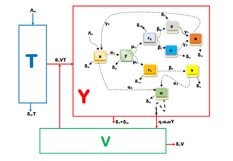
Multiscale modelling is a promising quantitative approach for studying infectious disease dynamics. This approach garners attention from both individuals who model diseases and those who plan for public health because it has great potential to contribute in expanding the understanding necessary for managing, reducing, and potentially exterminating infectious diseases. In this article, we developed a nested multiscale model of hepatitis B virus (HBV) that integrates the within-cell scale and the between-cell scale at cell level of organization of this disease system. The between-cell scale is linked to the within-cell scale by a once off inflow of initial viral infective inoculum dose from the between-cell scale to the within-cell scale through the process of infection; the within-cell scale is linked to the between-cell scale through the outflow of the virus from the within-cell scale to the between-cell scale through the process of viral shedding or excretion. The resulting multiple scales model is bidirectionally coupled in such a way that the within-cell scale and between-cell scale sub-models mutually affect each other, creating a reciprocal relationship. The computed reproductive number from the multiscale model confirms that the within-host scale and the between-host scale influence each other in a reciprocal manner. Numerical simulations are presented that also confirm the theoretical results and support the initial assumption that the within-cell scale and the between-cell scale influence each other in a reciprocal manner. This multiple scales modeling approach serves as a valuable tool for assessing the impact and success of health strategies aimed at controlling hepatitis B virus disease system.
Citation: Huguette Laure Wamba Makeng, Ivric Valaire Yatat-Djeumen, Bothwell Maregere, Rendani Netshikweta, Jean Jules Tewa, Winston Garira. Multiscale modelling of hepatitis B virus at cell level of organization[J]. Mathematical Biosciences and Engineering, 2024, 21(9): 7165-7193. doi: 10.3934/mbe.2024317
Multiscale modelling is a promising quantitative approach for studying infectious disease dynamics. This approach garners attention from both individuals who model diseases and those who plan for public health because it has great potential to contribute in expanding the understanding necessary for managing, reducing, and potentially exterminating infectious diseases. In this article, we developed a nested multiscale model of hepatitis B virus (HBV) that integrates the within-cell scale and the between-cell scale at cell level of organization of this disease system. The between-cell scale is linked to the within-cell scale by a once off inflow of initial viral infective inoculum dose from the between-cell scale to the within-cell scale through the process of infection; the within-cell scale is linked to the between-cell scale through the outflow of the virus from the within-cell scale to the between-cell scale through the process of viral shedding or excretion. The resulting multiple scales model is bidirectionally coupled in such a way that the within-cell scale and between-cell scale sub-models mutually affect each other, creating a reciprocal relationship. The computed reproductive number from the multiscale model confirms that the within-host scale and the between-host scale influence each other in a reciprocal manner. Numerical simulations are presented that also confirm the theoretical results and support the initial assumption that the within-cell scale and the between-cell scale influence each other in a reciprocal manner. This multiple scales modeling approach serves as a valuable tool for assessing the impact and success of health strategies aimed at controlling hepatitis B virus disease system.

| [1] | L. Christian, World Health Organization Statistics 2015, 2015. Available from: https://apps.who.int/mediacentre/news/releases/2015/world-health-statistics-2015/fr/index.html. |
| [2] |
M. Kane, Global programme for control of hepatitis B infection, Vaccine, 13 (1995), S47–S49. https://doi.org/10.1016/0264-410X(95)80050-N doi: 10.1016/0264-410X(95)80050-N

|
| [3] | A. A. Fall, Études de quelques modèles épidémiologiques: application à la transmission du virus de l'hépatite B en Afrique subsaharienne (cas du Sénégal), Ph.D thesis, Paul Verlaine-Metz University/Universite Gaston Berger, 2010. |
| [4] | N. Otric, Cameroon Health Among the 17 Countries Most Affected by Hepatitis, 2017. Available from: https://www.cameroon-info.net/article/cameroun-sante-le-cameroun-parmi-les-17-pays-les-plus-touches-par-lhepatite-selon-296589.html. |
| [5] |
G. M. Prifti, D. Moianos, E. Giannakopoulou, V. Pardali, J. E. Tavis, G. Zoidis, Recent advances in hepatitis B treatment, Pharmaceuticals, 14 (2021), 417. https://doi.org/10.3390/ph14050417 doi: 10.3390/ph14050417
|
| [6] |
C. W. Shepard, E. P. Simard, L. Finelli, A. E. Fiore, B. P. Bell, Hepatitis B virus infection: epidemiology and vaccination, Epidemiol. Rev., 28 (2006), 112–125. https://doi.org/10.1093/epirev/mxj009 doi: 10.1093/epirev/mxj009
|
| [7] | M. Matshidiso, Cameroon–The Government Aims to Lower to 53 the Prevalence Rate of Hepatitis B, 2020. Available from: https://actucameroun.com/2020/09/04/cameroun-le-gouvernement-ambitionne-de-baisser-a-53-le-taux-de-prevalence-de-lhepatite-b/. |
| [8] | B. A. Collins, D. Meenakshi, O. Sakuya, 91 million Africans infected with hepatitis B or C, 2022. Available from: https://www.afro.who.int/fr/news/91-millions-dafricains-infectes-par-lhepatite-b-ou-c. |
| [9] |
W. Garira, B. Maregere, The transmission mechanism theory of disease dynamics: Its aims, assumptions and limitations, Infect. Dis. Model., 8 (2023), 122–144. https://doi.org/10.1016/j.idm.2022.12.001 doi: 10.1016/j.idm.2022.12.001
|
| [10] |
W. Garira, K. Muzhinji, Application of the replication–transmission relativity theory in the development of multiscale models of infectious disease dynamics, J. Biol. Dyn., 17 (2023), 2255066. https://doi.org/10.1080/17513758.2023.2255066 doi: 10.1080/17513758.2023.2255066
|
| [11] |
W. Garira, The replication-transmission relativity theory for multiscale modelling of infectious disease systems, Sci. Rep., 9 (2019), 16353. https://doi.org/10.1038/s41598-019-52820-3 doi: 10.1038/s41598-019-52820-3
|
| [12] |
W. Garira, The research and development process for multiscale models of infectious disease systems, PLoS Comput. Biol., 16 (2020), e1007734. https://doi.org/10.1371/journal.pcbi.1007734 doi: 10.1371/journal.pcbi.1007734
|
| [13] |
M. A. Novak, S. Bonhoeffer, A. M. Hill, R. Boehme, H. C. Thomas, H. McDade, Viral dynamics in hepatitis B virus infection, Proc. Natl. Acad. Sci. USA, 93 (1996), 4398–4402. https://doi.org/10.1073/pnas.93.9.4398 doi: 10.1073/pnas.93.9.4398
|
| [14] |
A. V. Herz, S. Bonhoeffer, R. M. Anderson, R. M. May, M. A. Nowak, Viral dynamics in vivo: limitations on estimates of intracellular delay and virus decay, Proc. Natl. Acad. Sci. USA, 93 (1996), 7247–7251. https://doi.org/10.1073/pnas.93.14.7247 doi: 10.1073/pnas.93.14.7247
|
| [15] |
S. Zeuzem, A. Robert, P. Honkoop, W. K. Roth, S. W. Schalm, J. M. Schmidt, Dynamics of hepatitis B virus infection in vivo, J. Hepatol., 27 (1997), 431–436. https://doi.org/10.1016/S0168-8278(97)80345-5 doi: 10.1016/S0168-8278(97)80345-5
|
| [16] |
G. K. Lau, M. Tsiang, J. Hou, S. T. Yuen, W. F. Carman, L. Zhang, et al., Combination therapy with lamivudine and famciclovir for chronic hepatitis B–infected Chinese patients: a viral dynamics study, Hepatology, 32 (2000), 394–399. https://doi.org/10.1053/jhep.2000.9143 doi: 10.1053/jhep.2000.9143
|
| [17] |
S. R. Lewin, R. M. Ribeiro, T. Walters, G. K. Lau, S. Bowden, S. Locarnini, et al., Analysis of hepatitis B viral load decline under potent therapy: complex decay profiles observed, Hepatology, 34 (2001), 1012–1020. https://doi.org/10.1053/jhep.2001.28509 doi: 10.1053/jhep.2001.28509
|
| [18] |
N. Moolla, M. Kew, P. Arbuthnot, Regulatory elements of hepatitis B virus transcription, J. Viral Hepatitis, 9 (2002), 323–331. https://doi.org/10.1046/j.1365-2893.2002.00381.x doi: 10.1046/j.1365-2893.2002.00381.x
|
| [19] | V. Bruss, Hepatitis B virus morphogenesis, World J. Gastroenterol., 13 (2007), 65. |
| [20] |
J. Nakabayashi, A. Sasaki, A mathematical model of the intracellular replication and within host evolution of hepatitis type B virus: Understanding the long time course of chronic hepatitis, J. Theor. Biol., 269 (2011), 318–329. https://doi.org/10.1016/j.jtbi.2010.10.024 doi: 10.1016/j.jtbi.2010.10.024
|
| [21] |
J. Nakabayashi, The intracellular dynamics of hepatitis B virus (HBV) replication with reproduced virion "re-cycling", J. Theor. Biol., 396 (2016), 154–162. http://dx.doi.org/10.1016/j.jtbi.2016.02.008 doi: 10.1016/j.jtbi.2016.02.008
|
| [22] |
W. Garira, A complete categorization of multiscale models of infectious disease systems, J. Biol. Dyn., 11 (2017), 378–435. https://doi.org/10.1080/17513758.2017.1367849 doi: 10.1080/17513758.2017.1367849
|
| [23] |
W. Garira, A primer on multiscale modelling of infectious disease systems, Infect. Dis. Model., 3 (2018), 176–191. https://doi.org/10.1016/j.idm.2018.09.005 doi: 10.1016/j.idm.2018.09.005
|
| [24] |
W. Garira, D. Mathebula, A coupled multiscale model to guide malaria control and elimination, J. Theor. Biol., 475 (2019), 34–59. https://doi.org/10.1016/j.jtbi.2019.05.011 doi: 10.1016/j.jtbi.2019.05.011
|
| [25] |
W. Garira, M. C. Mafunda, From individual health to community health: towards multiscale modeling of directly transmitted infectious disease systems, J. Biol. Syst., 27 (2019), 131–166. https://doi.org/10.1142/S0218339019500074 doi: 10.1142/S0218339019500074
|
| [26] |
D. C. Krakauer, N. L. Komarova, Levels of selection in positive-strand virus dynamics, J. Evolution. Biol., 16 (2003), 64–73. https://doi.org/10.1046/j.1420-9101.2003.00481.x doi: 10.1046/j.1420-9101.2003.00481.x
|
| [27] |
R. Netshikweta, W. Garira, A nested multiscale model to study paratuberculosis in ruminants, Front. Appl. Math. Stat., 8 (2022), 817060. https://doi.org/10.3389/fams.2022.817060 doi: 10.3389/fams.2022.817060
|
| [28] |
R. Netshikweta, W. Garira, An embedded multiscale modelling to guide control and elimination of paratuberculosis in ruminants, Comput. Math. Methods M., 2021 (2021), 9919700. https://doi.org/10.1155/2021/9919700 doi: 10.1155/2021/9919700
|
| [29] |
L. Rong, J. Guedj, H. Dahari, D. J. Coffield Jr, M. Levi, P. Smith, et al., Analysis of hepatitis C virus decline during treatment with the protease inhibitor danoprevir using a multiscale model, PLoS Comput. Biol., 9 (2013), e1002959. https://doi.org/10.1371/journal.pcbi.1002959 doi: 10.1371/journal.pcbi.1002959
|
| [30] |
I. Hosseini, F. Mac Gabhann, Multi-scale modeling of HIV infection in vitro and APOBEC3G-based anti-retroviral therapy, PLoS Comput. Biol., 8 (2012), e1002371. https://doi.org/10.1371/journal.pcbi.1002371 doi: 10.1371/journal.pcbi.1002371
|
| [31] |
G. W. Suryawanshi, A. Hoffmann, A multi-scale mathematical modeling framework to investigate anti-viral therapeutic opportunities in targeting HIV-1 accessory proteins, J. Theor. Biol., 386 (2015), 89–104. https://doi.org/10.1016/j.jtbi.2015.08.032 doi: 10.1016/j.jtbi.2015.08.032
|
| [32] |
J. Guedj, A. U. Neumann, Understanding hepatitis C viral dynamics with direct-acting antiviral agents due to the interplay between intracellular replication and cellular infection dynamics, J. Theor. Biol., 267 (2010), 330–340. https://doi.org/10.1016/j.jtbi.2010.08.036 doi: 10.1016/j.jtbi.2010.08.036
|
| [33] |
E. L. Haseltine, J. B. Rawlings, J. Yin, Dynamics of viral infections: incorporating both the intracellular and extracellular levels, Comput. Chem. Eng., 29 (2005), 675–686. https://doi.org/10.1016/j.compchemeng.2004.08.022 doi: 10.1016/j.compchemeng.2004.08.022
|
| [34] | P. Van den Driessche, J. Watmough, Reproduction numbers and sub-threshold endemic equilibria for compartmental models of disease transmission, Math. Biosci., 180 (2002), 29–48. https://doi.org/10.1016/S0025-5564(02)00108-6 |
| [35] | P. Van den Driessche, J. Watmough, Further notes on the basic reproduction number, in Mathematical Epidemiology, Springer, (2008), 159–178. https://doi.org/10.1007/978-3-540-78911-6_6 |
| [36] | M. M. Ojo, F. O. Akinpelu, Lyapunov functions and global properties of seir epidemic model, Int. J. Chem. Math. Phys., 1 (2017), 11–16. |
| [37] |
W. Garira, K. Muzhinji, The universal theory for multiscale modelling of infectious disease dynamics, Mathematics, 11 (2023), 3874. https://doi.org/10.3390/math11183874 doi: 10.3390/math11183874
|
Figures(8) / Tables(2)

Huguette Laure Wamba Makeng, Ivric Valaire Yatat-Djeumen, Bothwell Maregere, Rendani Netshikweta, Jean Jules Tewa, Winston Garira. Multiscale modelling of hepatitis B virus at cell level of organization[J]. Mathematical Biosciences and Engineering, 2024, 21(9): 7165-7193. doi: 10.3934/mbe.2024317


 DownLoad: