With the growth of online networks, understanding the intricate structure of communities has become vital. Traditional community detection algorithms, while effective to an extent, often fall short in complex systems. This study introduced a meta-heuristic approach for community detection that leveraged a memetic algorithm, combining genetic algorithms (GA) with the stochastic hill climbing (SHC) algorithm as a local optimization method to enhance modularity scores, which was a measure of the strength of community structure within a network. We conducted comprehensive experiments on five social network datasets (Zachary's Karate Club, Dolphin Social Network, Books About U.S. Politics, American College Football, and the Jazz Club Dataset). Also, we executed an ablation study based on modularity and convergence speed to determine the efficiency of local search. Our method outperformed other GA-based community detection methods, delivering higher maximum and average modularity scores, indicative of a superior detection of community structures. The effectiveness of local search was notable in its ability to accelerate convergence toward the global optimum. Our results not only demonstrated the algorithm's robustness across different network complexities but also underscored the significance of local search in achieving consistent and reliable modularity scores in community detection.
Citation: Dongwon Lee, Jingeun Kim, Yourim Yoon. Improving modularity score of community detection using memetic algorithms[J]. AIMS Mathematics, 2024, 9(8): 20516-20538. doi: 10.3934/math.2024997
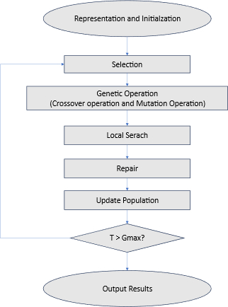
With the growth of online networks, understanding the intricate structure of communities has become vital. Traditional community detection algorithms, while effective to an extent, often fall short in complex systems. This study introduced a meta-heuristic approach for community detection that leveraged a memetic algorithm, combining genetic algorithms (GA) with the stochastic hill climbing (SHC) algorithm as a local optimization method to enhance modularity scores, which was a measure of the strength of community structure within a network. We conducted comprehensive experiments on five social network datasets (Zachary's Karate Club, Dolphin Social Network, Books About U.S. Politics, American College Football, and the Jazz Club Dataset). Also, we executed an ablation study based on modularity and convergence speed to determine the efficiency of local search. Our method outperformed other GA-based community detection methods, delivering higher maximum and average modularity scores, indicative of a superior detection of community structures. The effectiveness of local search was notable in its ability to accelerate convergence toward the global optimum. Our results not only demonstrated the algorithm's robustness across different network complexities but also underscored the significance of local search in achieving consistent and reliable modularity scores in community detection.

| [1] | P. Bedi, C. Sharma, Community detection in social networks, Wiley interdisciplinary reviews: Data mining and knowledge discovery, 6 (2016), 115–135. https://doi.org/10.1002/widm.1178 |
| [2] | L. M. Naeni, R. Berretta, P. Moscato, MA-Net: A reliable memetic algorithm for community detection by modularity optimization, In Proceedings of the 18th Asia Pacific Symposium on Intelligent and Evolutionary Systems, 1 (2015), Springer. https://doi.org/10.1007/978-3-319-13359-1_25 |
| [3] |
R. K. Behera, D. Naik, S. K. Rath, R. Dharavath, Genetic algorithm-based community detection in large-scale social networks, Neural Comput. Appl., 32 (2020), 9649–9665. https://doi.org/10.1007/s00521-019-04487-0 doi: 10.1007/s00521-019-04487-0

|
| [4] |
E. Ferrara, A large-scale community structure analysis in Facebook, EPJ Data Sci., 1 (2012), 1–30. https://doi.org/10.1140/epjds9 doi: 10.1140/epjds9
|
| [5] | J. Goldenberg, B. Libai, E. Muller, Using complex systems analysis to advance marketing theory development: Modeling heterogeneity effects on new product growth through stochastic cellular automata, Acad. Mark. Sci. Rev., 9 (2001), 1–18. |
| [6] |
M. E. Newman, M. Girvan, Finding and evaluating community structure in networks, Phys. Rev. E, 69 (2004), 026113. https://doi.org/10.1103/PhysRevE.69.026113 doi: 10.1103/PhysRevE.69.026113
|
| [7] |
A. Pothen, H. D. Simon, K. P. Liou, Partitioning sparse matrices with eigenvectors of graphs, SIAM J. Matrix Anal. A, 11(1990), 430–452. https://doi.org/10.1137/0611030 doi: 10.1137/0611030
|
| [8] |
M. Girvan, M. E. Newman, Community structure in social and biological networks, P. Natl Acad. Sci., 99 (2002), 7821–7826. https://doi.org/10.1073/pnas.122653799 doi: 10.1073/pnas.122653799
|
| [9] |
U. Brandes, D. Delling, M. Gaertler, R. Gorke, M. Hoefer, Z. Nikoloski, et al., On modularity clustering, IEEE T. Knowl. Data En., 20 (2007), 172–188. https://doi.org/10.1109/TKDE.2007.190689 doi: 10.1109/TKDE.2007.190689
|
| [10] | K. Wakita, T. Tsurumi, Finding community structure in mega-scale social networks, In Proceedings of the 16th international conference on World Wide Web, 2007. https://doi.org/10.1145/1242572.1242805 |
| [11] |
I. Koc, A fast community detection algorithm based on coot bird metaheuristic optimizer in social networks, Eng. Appl. Artif. Intel., 114 (2022), 105202. https://doi.org/10.1016/j.engappai.2022.105202 doi: 10.1016/j.engappai.2022.105202
|
| [12] |
Y. Zhang, Y. G. Liu, J. T. Li, J. J. Zhu, C. H. Yang, W. Yang, et al., WOCDA: A whale optimization based community detection algorithm, Physica A, 539 (2020), 122937. https://doi.org/10.1016/j.physa.2019.122937 doi: 10.1016/j.physa.2019.122937
|
| [13] | C. Pizzuti, Ga-net: A genetic algorithm for community detection in social networks, In International conference on parallel problem solving from nature, Springer, 2008. https://doi.org/10.1007/978-3-540-87700-4_107 |
| [14] |
X. Zeng, W. Wang; C. Chen, G. G. Yen, A consensus community-based particle swarm optimization for dynamic community detection, IEEE T. Cybernetics, 50 (2019), 2502–2513. https://doi.org/10.1109/TCYB.2019.2938895 doi: 10.1109/TCYB.2019.2938895
|
| [15] | C. Honghao, F. Zuren, R. Zhigang, Community detection using ant colony optimization, In 2013 IEEE congress on evolutionary computation, 2013. |
| [16] | M. Tasgin, A. Herdagdelen, H. Bingol, Community detection in complex networks using genetic algorithms, arXiv: 0711.0491, 2007. |
| [17] |
M. Gong, B. Fu, L. C. Jiao, H. F. Du, Memetic algorithm for community detection in networks, Phys. Rev. E, 84 (2011), 056101. https://doi.org/10.1103/PhysRevE.84.056101 doi: 10.1103/PhysRevE.84.056101
|
| [18] |
R. Shang, J. Bai, L. C. Jiao, C. Jin, Community detection based on modularity and an improved genetic algorithm, Physica A, 392 (2013), 1215–1231. https://doi.org/10.1016/j.physa.2012.11.003 doi: 10.1016/j.physa.2012.11.003
|
| [19] |
Y. Liang, L. Wang, Applying genetic algorithm and ant colony optimization algorithm into marine investigation path planning model, Soft Comput., 24 (2020), 8199–8210. https://doi.org/10.1007/s00500-019-04414-4 doi: 10.1007/s00500-019-04414-4
|
| [20] | K. De Jong, Genetic algorithms: A 10 year perspective, In Proceedings of the first International Conference on Genetic Algorithms and their Applications, Psychology Press, 2014. |
| [21] |
P. Preux, E. G. Talbi, Towards hybrid evolutionary algorithms, Int. T. Oper. Res., 6 (1999), 557–570. https://doi.org/10.1111/j.1475-3995.1999.tb00173.x doi: 10.1111/j.1475-3995.1999.tb00173.x
|
| [22] | T. A. El-Mihoub, A. A. Hopgood, N. Lars, B. Alan, Hybrid genetic algorithms: A review, Eng. Lett., 13 (2006), 124–137. |
| [23] |
M. E. Newman, Fast algorithm for detecting community structure in networks, Phys. Rev. E, 69 (2004), 066133. https://doi.org/10.1103/PhysRevE.69.066133 doi: 10.1103/PhysRevE.69.066133
|
| [24] | J. Holland, Adaptation in natural and artificial systems, Applying genetic algorithm to increase the efficiency of a data flow-based test data generation approach, the university of michigan press, Ann. Arbor. 1975, 1–5. |
| [25] | L. Haldurai, T. Madhubala, R. Rajalakshmi, A study on genetic algorithm and its applications, Int. J. Comput. Sci. Eng., 4 (2016), 139. |
| [26] | W. E. Hart, N. Krasnogor, J. E. Smith, Memetic evolutionary algorithms, In Recent Advances in Memetic Algorithms, Springer, 2005, 3–27. https://doi.org/10.1007/3-540-32363-5_1 |
| [27] | P. Moscato, C. Cotta, A gentle introduction to memetic algorithms, In Handbook of metaheuristics, Springer, 2003,105–144. https://doi.org/10.1007/0-306-48056-5_5 |
| [28] |
N. Krasnogor, J. Smith, A tutorial for competent memetic algorithms: Model, taxonomy, and design issues, IEEE T. Evolut. Comput., 9 (2005), 474–488. https://doi.org/10.1109/TEVC.2005.850260 doi: 10.1109/TEVC.2005.850260
|
| [29] |
G. Acampora, V. Loia, S. Salerno, A. Vitiello, A hybrid evolutionary approach for solving the ontology alignment problem, Int. J. Intel. Syst., 27 (2012), 189–216. https://doi.org/10.1002/int.20517 doi: 10.1002/int.20517
|
| [30] |
R. Cabido, A. S. Montemayor, J. J. Pantrigo, High performance memetic algorithm particle filter for multiple object tracking on modern GPUs, Soft Comput., 16(2012), 217–230. https://doi.org/10.1007/s00500-011-0715-2 doi: 10.1007/s00500-011-0715-2
|
| [31] |
Y. Li, J. Liu, C. Liu, A comparative analysis of evolutionary and memetic algorithms for community detection from signed social networks, Soft Comput., 18 (2014), 329–348. https://doi.org/10.1007/s00500-013-1060-4 doi: 10.1007/s00500-013-1060-4
|
| [32] |
B. Yang, W. Cheung, J. Liu, Community mining from signed social networks, IEEE T. Knowl. Data En., 19 (2007), 1333–1348. https://doi.org/10.1109/TKDE.2007.1061 doi: 10.1109/TKDE.2007.1061
|
| [33] |
P. Doreian, A multiple indicator approach to blockmodeling signed networks, Soc. Networks, 30 (2008), 247–258. https://doi.org/10.1016/j.socnet.2008.03.005 doi: 10.1016/j.socnet.2008.03.005
|
| [34] |
V. A. Traag, J. Bruggeman, Community detection in networks with positive and negative links, Phys. Rev. E, 80 (2009), 036115. https://doi.org/10.1103/PhysRevE.80.036115 doi: 10.1103/PhysRevE.80.036115
|
| [35] | L. Wu, X. Ying, X. Wu, A. Lu, Z. H. Zhou, Spectral analysis of k-balanced signed graphs, In Advances in Knowledge Discovery and Data Mining: 15th Pacific-Asia Conference, PAKDD 2011, Shenzhen, China, May 24-27, 2011, Proceedings, Part Ⅱ 15. 2011. Springer. |
| [36] |
S. Ranjkesh, B. Masoumi, S. M. Hashemi, A novel robust memetic algorithm for dynamic community structures detection in complex networks, World Wide Web, 27 (2024), 3. https://doi.org/10.1007/s11280-024-01238-7 doi: 10.1007/s11280-024-01238-7
|
| [37] |
M. Miao, J. R. Wu, F. J. Cai, Y. G. Wang, A modified memetic algorithm with an application to gene selection in a sheep body weight study, Animals, 12 (2022), 201. https://doi.org/10.3390/ani12020201 doi: 10.3390/ani12020201
|
| [38] |
J. Andre, P. Siarry, T. Dognon, An improvement of the standard genetic algorithm fighting premature convergence in continuous optimization, Adv. Eng. Softw., 32 (2001), 49–60. https://doi.org/10.1016/S0965-9978(00)00070-3 doi: 10.1016/S0965-9978(00)00070-3
|
| [39] |
Y. D. Kwon, S. B. Kwon, S. B. Jin, J. Y. Kim, Convergence enhanced genetic algorithm with successive zooming method for solving continuous optimization problems, Comput. Struct., 81 (2003), 1715–1725. https://doi.org/10.1016/S0045-7949(03)00183-4 doi: 10.1016/S0045-7949(03)00183-4
|
| [40] | T. F. Gonzalez, Handbook of approximation algorithms and metaheuristics, 2007: Chapman and Hall/CRC. |
| [41] | C. H. Papadimitriou, K. Steiglitz, Combinatorial optimization: Algorithms and complexity, Courier Corporation, 1998. |
| [42] | E. Aarts, J. H. Korst, P. J. Laarhoven, Simulated annealing, E. Aarts, JK Lenstra, eds., Local Search in Combinatorial Optimization, John Wiley and Sons, New York, NY, 91120 (1997). |
| [43] | S. J. Russell, P. Norvig, Artificial intelligence: A modern approach, Pearson, 2016. |
| [44] |
B. Mondal, K. Dasgupta, P. Dutta, Load balancing in cloud computing using stochastic hill climbing-a soft computing approach, Procedia Technol., 4 (2012), 783–789. https://doi.org/10.1016/j.protcy.2012.05.128 doi: 10.1016/j.protcy.2012.05.128
|
| [45] | B. L. Miller, D. E. Goldberg, Genetic algorithms, tournament selection, and the effects of noise, Complex Syst., 9 (1995), 193–212. |
| [46] | R. Halalai, C. Lemnaru, R. Potolea, Distributed community detection in social networks with genetic algorithms, In Proceedings of the 2010 IEEE 6th International Conference on Intelligent Computer Communication and Processing, 2010. https://doi.org/10.1109/ICCP.2010.5606467 |
| [47] | D. E. Goldberg, Genetic algorithms in search, optimization and machine learning, Addison-Wesley Longman Publishing Co., Inc. 1989. |
| [48] |
W. W. Zachary, An information flow model for conflict and fission in small groups, J. Anthropol. Res., 33 (1977), 452–473. https://doi.org/10.1086/jar.33.4.3629752 doi: 10.1086/jar.33.4.3629752
|
| [49] |
J. Q. Jiang, L. J. McQuay, Modularity functions maximization with nonnegative relaxation facilitates community detection in networks, Physica A, 391 (2012), 854–865. https://doi.org/10.1016/j.physa.2011.08.043 doi: 10.1016/j.physa.2011.08.043
|
| [50] |
D. Lusseau, K. Schneider, O. J. Boisseau, P. Haase, E. Slooten, S. M. Dawson, The bottlenose dolphin community of doubtful sound features a large proportion of long-lasting associations: Can geographic isolation explain this unique trait? Behav. Ecol. Sociobiol., 54 (2003), 396–405. https://doi.org/10.1007/s00265-003-0651-y doi: 10.1007/s00265-003-0651-y
|
| [51] |
M. E. Newman, Modularity and community structure in networks, P. Natl Acad. Sci., 103 (2006), 8577–8582. https://doi.org/10.1073/pnas.0601602103 doi: 10.1073/pnas.0601602103
|
| [52] | The red hot Jazz archive. Available from: http://www.redhotjazz.com. |
| [53] | C. Pizzuti, A multi-objective genetic algorithm for community detection in networks, In 2009 21st IEEE International Conference on Tools with Artificial Intelligence, 2009. https://doi.org/10.1109/ICTAI.2009.58 |
| [54] |
M. Guerrero, F. G. Montoya, R. Baños, A. Alcayde, C. Gil, Adaptive community detection in complex networks using genetic algorithms, Neurocomputing, 266 (2017), 101–113. https://doi.org/10.1016/j.neucom.2017.05.029 doi: 10.1016/j.neucom.2017.05.029
|
| [55] | C. Shi, W. Yi, B. Wu, C. Zhong, A new genetic algorithm for community detection, In Complex Sciences: First International Conference, Complex 2009, Shanghai, China, February 23-25, 2009, Revised Papers, Part 2, Springer, 2009. https://doi.org/10.1007/978-3-642-02469-6_11 |
| [56] | R. Zheng, A fast community detection algorithm based on clustering coefficient, In 3rd International Conference on Mechatronics Engineering and Information Technology (ICMEIT 2019), Atlantis Press, 2019. https://doi.org/10.2991/icmeit-19.2019.100 |
| [57] | D. Choudhury, S. Bhattacharjee, A. Das, An empirical study of community and sub-community detection in social networks applying Newman-Girvan algorithm, In 2013 1st international conference on emerging trends and applications in computer science, IEEE, 2013. https://doi.org/10.1109/ICETACS.2013.6691399 |
| [58] | N. Du, B. Wu, X. Pei, Community detection in large-scale social networks, In Proceedings of the 9th WebKDD and 1st SNA-KDD 2007 workshop on Web mining and social network analysis, 2007. |
| [59] |
A. Said, R. A. Abbasi, O. Maqbool, A. Daud, N. R. Aljohani, CC-GA: A clustering coefficient based genetic algorithm for detecting communities in social networks, Appl. Soft Comput., 63 (2018), 59–70. https://doi.org/10.1016/j.asoc.2017.11.014 doi: 10.1016/j.asoc.2017.11.014
|
| [60] | W. Y. Lin, W. Y. Lee, T. P. Hong, Adapting crossover and mutation rates in genetic algorithms, J. Inf. Sci. Eng., 19 (2003), 889–903. |
| [61] |
A. Clauset, M. E. Newman, C. Moore, Finding community structure in very large networks, Phys. Rev. E, 70 (2004), 066111. https://doi.org/10.1103/PhysRevE.70.066111 doi: 10.1103/PhysRevE.70.066111
|
| [62] |
S. Wang, J. Liu, Constructing robust community structure against edge-based attacks, IEEE Syst. J., 13 (2018), 582–592. https://doi.org/10.1109/JSYST.2018.2835642 doi: 10.1109/JSYST.2018.2835642
|
| [63] |
S. Wang, J. Liu, X. Wang, Mitigation of attacks and errors on community structure in complex networks, J. Stat. Mech.-Theory E., 2017 (2017), 043405. https://doi.org/10.1088/1742-5468/aa6581 doi: 10.1088/1742-5468/aa6581
|
| [64] |
S. Wang, J. Liu, Community robustness and its enhancement in interdependent networks, Appl. Soft Comput., 77 (2019), 665–677. https://doi.org/10.1016/j.asoc.2019.01.045 doi: 10.1016/j.asoc.2019.01.045
|
| [65] |
V. D. F. Vieira, C. R. Xavier, A. G. Evsukoff, A comparative study of overlapping community detection methods from the perspective of the structural properties, Appl. Netw. Sci., 5 (2020), 1–42. https://doi.org/10.1007/s41109-020-00289-9 doi: 10.1007/s41109-020-00289-9
|
| [66] |
L. Danon, A. Díaz-Guilera1, J. Duch, A. Arenas, Comparing community structure identification, J. Stat. Mech.-Theory E., 2005 (2005), P09008. https://doi.org/10.1088/1742-5468/2005/09/P09008 doi: 10.1088/1742-5468/2005/09/P09008
|
| [67] |
L. M. Collins, C. W. Dent, Omega: A general formulation of the rand index of cluster recovery suitable for non-disjoint solutions, Multivar. Behav. Res., 23 (1988), 231–242. https://doi.org/10.1207/s15327906mbr2302_6 doi: 10.1207/s15327906mbr2302_6
|
| [68] |
M. Li, J. Liu, A link clustering based memetic algorithm for overlapping community detection, Physica A, 503 (2018), 410–423. https://doi.org/10.1016/j.physa.2018.02.133 doi: 10.1016/j.physa.2018.02.133
|
| [69] |
H. Shen, X. Q. Cheng, K. Cai, M. B. Hu, Detect overlapping and hierarchical community structure in networks, Physica A, 388 (2009), 1706–1712. https://doi.org/10.1016/j.physa.2008.12.021 doi: 10.1016/j.physa.2008.12.021
|
| [70] | D. Jin, Z. Y. Liu, W. H. Li, D. X. He, W. X. Zhang, Graph convolutional networks meet markov random fields: Semi-supervised community detection in attribute networks, In Proceedings of the AAAI conference on artificial intelligence, 2019. https://doi.org/10.1609/aaai.v33i01.3301152 |
| [71] |
W. Shi, Network embedding via community based variational autoencoder, IEEE Access, 7 (2019), 25323–25333. https://doi.org/10.1109/ACCESS.2019.2900662 doi: 10.1109/ACCESS.2019.2900662
|


Figures(4) / Tables(6)

Dongwon Lee, Jingeun Kim, Yourim Yoon. Improving modularity score of community detection using memetic algorithms[J]. AIMS Mathematics, 2024, 9(8): 20516-20538. doi: 10.3934/math.2024997


 DownLoad: