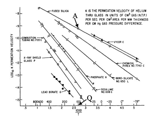
Although the densities of crystal quartz and vitreous silica differ only by about 17% (2.65 and 2.20 g/cm3, respectively), the helium permeability of silica glass is six orders more elevated than that of crystal quartz. This vast difference has puzzled researchers for decades considering that silica glass and quartz crystal have the same chemical composition. This work discusses the mechanism of high helium permeation through silica glass. It briefly reviews the experimental data and its contradictions with the continuous random network theory. A recently proposed nanoflake model for silica glass structure is utilized to explain the origin of glass permeation to helium. According to the nanoflake model, the formation of nanoflakes not only brings a one-dimensional medium-range ordering structure into silica glass but simultaneously creates regions where van der Waals bonds replace the oxygen-silicon covalent bonds. It is the weakness of van der Waals bonds that causes the helium mobility in these areas to increase.
Citation: Shangcong Cheng. On the mechanism of helium permeation through silica glass[J]. AIMS Materials Science, 2024, 11(3): 438-448. doi: 10.3934/matersci.2024022
Although the densities of crystal quartz and vitreous silica differ only by about 17% (2.65 and 2.20 g/cm3, respectively), the helium permeability of silica glass is six orders more elevated than that of crystal quartz. This vast difference has puzzled researchers for decades considering that silica glass and quartz crystal have the same chemical composition. This work discusses the mechanism of high helium permeation through silica glass. It briefly reviews the experimental data and its contradictions with the continuous random network theory. A recently proposed nanoflake model for silica glass structure is utilized to explain the origin of glass permeation to helium. According to the nanoflake model, the formation of nanoflakes not only brings a one-dimensional medium-range ordering structure into silica glass but simultaneously creates regions where van der Waals bonds replace the oxygen-silicon covalent bonds. It is the weakness of van der Waals bonds that causes the helium mobility in these areas to increase.

| [1] |
Bruckner R (1971) Properties and structure of vitreous silica. Ⅱ. J Non-Cryst Solids 5: 177–216. https://doi.org/10.1016/0022-3093(71)90032-9 doi: 10.1016/0022-3093(71)90032-9

|
| [2] | Varshneya AK, Mauro JC (2019) Fundamentals of Inorganic Glasses, 3rd Eds, Amsterdam: Elsevier. https://doi.org/10.1016/C2017-0-04281-7 |
| [3] | Doremus RH (1994) Glass Science, 2nd Eds, New Jersey: John Wiley & Sons, Inc. |
| [4] | Shelby JE (2005) Introduction to Glass Science and Technology, 2nd Eds, Cambridge: The Royal Society of Chemistry. |
| [5] |
Elsey HM (1926) The diffusion of helium and hydrogen through quartz glass at room temperature. J Am Chem Soc 48: 1600–1601. https://doi.org/10.1021/ja01417a501 doi: 10.1021/ja01417a501
|
| [6] |
Norton FJ (1953) Helium diffusion through glass. J Am Chem Soc 36: 90–96. https://doi.org/10.1111/j.1151-2916.1953.tb12843.x doi: 10.1111/j.1151-2916.1953.tb12843.x
|
| [7] |
Norton FJ (1957) Permeation of gases through solids. J Appl Phys 28: 34–39. https://doi.org/10.1063/1.1722570 doi: 10.1063/1.1722570
|
| [8] |
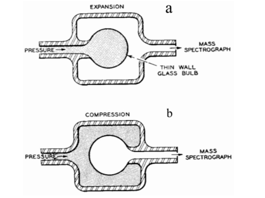
McAfee KB (1958) Stress‐enhanced diffusion in glass. Ⅰ. Glass under tension and compression. J Chem Phys 28: 218–226. https://doi.org/10.1063/1.1744096 doi: 10.1063/1.1744096
|
| [9] |
Leiby CC, Chen CL (1960) Diffusion coefficients, solubilities, and permeabilities for He, Ne, H2, and N2 in Vycor glass. J Appl Phys 31: 268–274. https://doi.org/10.1063/1.1735556 doi: 10.1063/1.1735556
|
| [10] |
Shelby JE (1973) Effect of phase separation on helium migration in sodium silicate glasses. J Am Ceram Soc 56: 263–266. https://doi.org/10.1111/j.1151-2916.1973.tb12484.x doi: 10.1111/j.1151-2916.1973.tb12484.x
|
| [11] |
Shelby JE (1974) Helium diffusion and solubility in K2O-SiO2 glasses. J Am Ceram Soc 57: 260–263. https://doi.org/10.1111/j.1151-2916.1974.tb10883.x doi: 10.1111/j.1151-2916.1974.tb10883.x
|
| [12] |
Hacarlioglu P, Lee D, Gibbs GV, et al. (2008) Activation energies for permeation of He and H2 through silica membranes: An ab initio calculation study. J Membrane Sci 313: 277–283. http://doi.org:10.1016/j.memsci.2008.01.018 doi: 10.1016/j.memsci.2008.01.018
|
| [13] |
Shackelford JF (2014) Gas solubility and diffusion in oxide glasses—implications for nuclear wasteforms. Procedia Mater Sci 7: 278–285. http://doi.org:10.1016/j.mspro.2014.10.036 doi: 10.1016/j.mspro.2014.10.036
|
| [14] |
Yoshioka T, Nakata A, Tung KL, et al. (2019) Molecular dynamics simulation study of solid vibration permeation in microporous amorphous silica network voids. Membranes 9: 132. http://doi.org:10.3390/membranes9100132 doi: 10.3390/membranes9100132
|
| [15] |
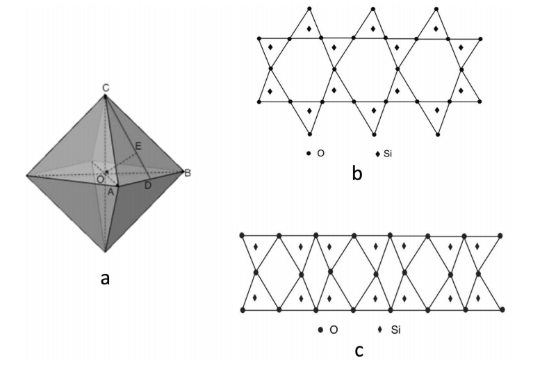
Cheng S (2017) A nanoflake model for the medium range structure in vitreous silica. Phys Chem Glasses-B 58: 33–40. https://doi.org/10.13036/17533562.57.2.104 doi: 10.13036/17533562.57.2.104
|
| [16] |
Cheng S (2022) Two-stage model of silicate glass transition. GJSFR 22: 1–9. http://doi.org/10.34257/GJSFRAVOL22IS7PG1 doi: 10.34257/GJSFRAVOL22IS7PG1
|
| [17] |
Zachariasen WH (1932) The atomic arrangement in glass. J Am Chem Soc 54: 3841–3851. https://doi.org/10.1021/ja01349a006 doi: 10.1021/ja01349a006
|
| [18] |
Warren BE (1934) X-ray determination of the glass structure. J Am Ceram Soc 17: 249–254. https://doi.org/10.1111/j.1151-2916.1934.tb19316.x doi: 10.1111/j.1151-2916.1934.tb19316.x
|
| [19] |
Warren BE, Biscoe J (1938) Fourier analysis of X-ray patterns of soda-silica glass. J Am Ceram Soc 21: 259–265. https://doi.org/10.1111/j.1151-2916.1938.tb15774.x doi: 10.1111/j.1151-2916.1938.tb15774.x
|
| [20] | Cheng S (2022) Research Advancements in the Field of Materials Science, London: Index of Sciences Ltd. |
| [21] |
Cheng S (2023) The origin of anomalous density behavior of silica glass. Materials 16: 6218. https://doi.org/10.3390/ma16186218. doi: 10.3390/ma16186218
|
| [22] |
Rayleigh L (1936) Studies on the passage of helium at ordinary temperature through glasses, crystals, and organic materials. P Roy Soc A-Math Phy 156: 350–357. https://doi.org/10.1098/rspa.1936.0152 doi: 10.1098/rspa.1936.0152
|
| [23] |
Rayleigh L (1937) An attempt to detect the passage of helium through a crystal lattice at high temperatures. P Roy Soc A-Math Phy 163: 376–380. https://doi.org/10.1098/RSPA.1937.0233 doi: 10.1098/RSPA.1937.0233
|
| [24] |
Greaves GN (1985) EXAFS and the structure of glass. J Non-Cryst Solids 71: 203–217. https://doi.org/10.1016/0022-3093(85)90289-3 doi: 10.1016/0022-3093(85)90289-3
|
| [25] |
Greaves GN, Fontaine A, Lagarde P, et al. (1981) Local structure of silicate glasses. Nature 293: 611–616. https://doi.org/10.1038/293611a0 doi: 10.1038/293611a0
|
| [26] |
Ojovan MI (2021) The modified random network (MRN) model within the configuron percolation theory (CPT) of glass transition. Ceramics 4: 121–134. https://doi.org/10.3390/ceramics4020011 doi: 10.3390/ceramics4020011
|
| [27] |
Israelachivili JN (1981) The force between surfaces. Philos Mag A 43: 753–770. http://doi.org/10.1080/01418618108240406 doi: 10.1080/01418618108240406
|
| [28] | Shelekhin AB, Dixon AG, Ma YH (1995) Theory of gas diffusion and permeation in inorganic molecular-sieve membranes. Aiche J 41: 58–67. https://aiche.onlinelibrary.wiley.com/doi/10.1002/aic.690410107 |
| [29] | Royal Society of Chemistry (2024) Available from: https://www.rsc.org/periodic-table/element/2/helium. |
| [30] |
Griffith A (1921) The phenomena of rupture and flow in solids. Philos T R Soc A 221: 163–198. https://doi.org/10.1098/rsta.1921.0006 doi: 10.1098/rsta.1921.0006
|
| [31] |
Otto WH (1955) Relationship of tensile strength of glass fibers to diameter. J Am Ceram Soc 38: 122–124. https://doi.org/10.1111/j.1151-2916.1955.tb14588.x doi: 10.1111/j.1151-2916.1955.tb14588.x
|
Figures(4)

Shangcong Cheng. On the mechanism of helium permeation through silica glass[J]. AIMS Materials Science, 2024, 11(3): 438-448. doi: 10.3934/matersci.2024022


 DownLoad: