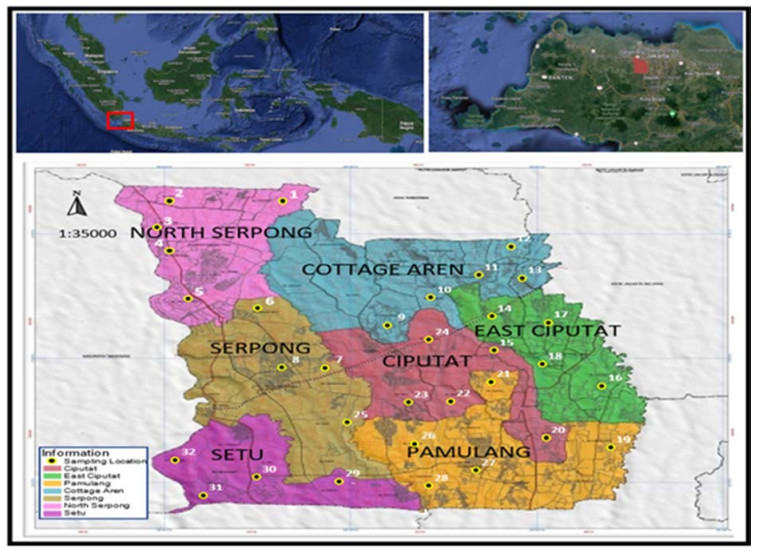
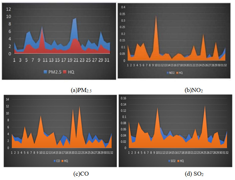
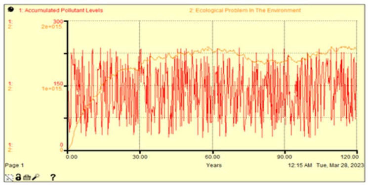
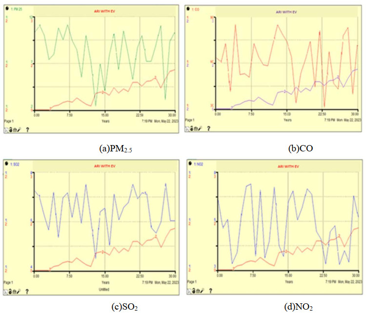
Increasing emissions from mobile sources have become a major focus in terms of health, environmental sustainability, and climate change. South Tangerang City is the Indonesian city with the highest yearly average pollution level. This study's objectives are to quantify the levels of pollutant concentrations that endanger human health and the environment and to devise a plan for reducing the pollution brought on by vehicle emissions. This study used an analytic observational research design. Data was taken from 32 points in 7 sub-districts in the city of South Tangerang with human and environmental samples. Human samples using the Hazard Quotient. Data is processed using Stella for the next 30 years. HQ value of PM2.5, NO2, SO2, and CO pollution has risen to greater than 1, endangering human health. CO and PM2.5, with HQ values of 3.315 and 1.644, both present serious health concerns. The accumulation of PM2.5, NO2, SO2, and CO pollutants over the next 30 years will have a substantial impact on South Tangerang's environmental conditions. South Tangerang could encourage the growth of a smart city by supporting the use of electric vehicles. Human health is at risk due to the increase in the HQ value of PM2.5, NO2, SO2, and CO pollution above 1. The environmental conditions in South Tangerang be significantly impacted by PM2.5, NO2, SO2, and CO pollutants over the ensuing 30 years. A mitigation strategy is needed in the form of smart transportation in the form of electric vehicles
Citation: Ernyasih, Anwar Mallongi, Anwar Daud, Sukri Palutturi, Stang, Abdul RazakThaha, Erniwati Ibrahim, Wesam Al Madhoun, Andriyani. Strategy formitigating health and environmental risks from vehicle emissions in SouthTangerang[J]. AIMS Environmental Science, 2023, 10(6): 794-808. doi: 10.3934/environsci.2023043
Increasing emissions from mobile sources have become a major focus in terms of health, environmental sustainability, and climate change. South Tangerang City is the Indonesian city with the highest yearly average pollution level. This study's objectives are to quantify the levels of pollutant concentrations that endanger human health and the environment and to devise a plan for reducing the pollution brought on by vehicle emissions. This study used an analytic observational research design. Data was taken from 32 points in 7 sub-districts in the city of South Tangerang with human and environmental samples. Human samples using the Hazard Quotient. Data is processed using Stella for the next 30 years. HQ value of PM2.5, NO2, SO2, and CO pollution has risen to greater than 1, endangering human health. CO and PM2.5, with HQ values of 3.315 and 1.644, both present serious health concerns. The accumulation of PM2.5, NO2, SO2, and CO pollutants over the next 30 years will have a substantial impact on South Tangerang's environmental conditions. South Tangerang could encourage the growth of a smart city by supporting the use of electric vehicles. Human health is at risk due to the increase in the HQ value of PM2.5, NO2, SO2, and CO pollution above 1. The environmental conditions in South Tangerang be significantly impacted by PM2.5, NO2, SO2, and CO pollutants over the ensuing 30 years. A mitigation strategy is needed in the form of smart transportation in the form of electric vehicles

| [1] |
Burnett R, Chen H, Szyszkowicz M., Fann, N, et al. (2018) Global estimates of mortality associated with longterm exposure to outdoor fine particulate matter. P Natl Acad Sci USA 115: 9592–9597. https://doi.org/10.1073/pnas.1803222115 doi: 10.1073/pnas.1803222115

|
| [2] |
He M, Zhong Y, Chen Y, et al. (2022) Association of short-term exposure to air pollution with emergency visits for respiratory diseases in children. IScience 25: 104879. https://doi.org/10.1016/j.isci.2022.104879 doi: 10.1016/j.isci.2022.104879
|
| [3] |
Song H, Deng Shun X, Lu Zhen Z, et al. (2021) Scenario analysis of vehicular emission abatement procedures in Xi'an, China. Environ Pollut 269: 116187. https://doi.org/10.1016/j.envpol.2020.116187 doi: 10.1016/j.envpol.2020.116187
|
| [4] |
Zeydan O, Zeydan I (2023) Impacts of travel bans and travel intention changes on aviation emissions due to Covid-19 pandemic. Environ Dev Sustain. https://doi.org/10.1007/s10668-023-02916-8 doi: 10.1007/s10668-023-02916-8
|
| [5] |
Rao S, Zheng Z, Yang C (2023) Effect of Cyclohexane on the combustion characteristics of Multi-Component Gasoline Surrogate Fuels. Molecules 28. https://doi.org/10.3390/ molecules28114273 doi: 10.3390/ molecules28114273
|
| [6] | Kumar Nallapaneni M, Dash A, (2017) The Internet of Things: An Opportunity for Transportation and Logistics. IEEE Int Conf Inven Comput Informatics (ICICI) 11: 194–197. https://www.researchgate.net/publication/321242420 |
| [7] |
Danish, Baloch Muhammad A, Suad S (2018) Modeling the impact of transport energy consumption on CO2 emission in Pakistan: Evidence from ARDL approach. Environ Sci Pollut Res 25: 9461–9473. https://doi.org/10.1007/s11356-018-1230-0 doi: 10.1007/s11356-018-1230-0
|
| [8] |
Mohd Shafie Siti H, Mahmud M (2020) Urban air pollutant from motor vehicle emissions in kuala lumpur, malaysia. Aerosol Air Qual Res 20: 2793–2804. https://doi.org/10.4209/aaqr.2020.02.0074 doi: 10.4209/aaqr.2020.02.0074
|
| [9] |
Bezyk Y, Gorka M, Sowka I, et al. (2023) Temporal Dynamic and Controlling Factors of CO2 and CH4 Variability in The Urban Atmosphere of Wroclaw, Poland. Sci Total Environ 12. https://doi.org/10.1016/j.scitotenv.2023.164771 doi: 10.1016/j.scitotenv.2023.164771
|
| [10] |
Nurjani E, Hafizha, K P, Purwanto D, Ulumia F, et al. (2021) Carbon Emissions from the Transportation Sector during the Covid-19 Pandemic in the Special Region of Yogyakarta, Indonesia. IOP Conf Series: Earth and Environ Sci 940: 0–7. https://doi.org/10.1088/1755-1315/940/1/012039 doi: 10.1088/1755-1315/940/1/012039
|
| [11] |
Gonzalez C M, Gomez C D, Rojas N Y, et al. (2017) Relative impact of on-road vehicular and point-source industrial emissions of air pollutants in a medium-sized Andean city. Atmos Environ 152: 279–289. https://doi.org/10.1016/j.atmosenv.2016.12.048 doi: 10.1016/j.atmosenv.2016.12.048
|
| [12] |
Teymouri P, Sarbakhsh P, Taghipour H, et al. (2023) Modeling fuel consumption and emissions by taxis in Tabriz, Iran: uncertainty and sensitivity analyses. Environ Sci Pollut Res 0123456789. https://doi.org/10.1007/s11356-023-27883-5 doi: 10.1007/s11356-023-27883-5
|
| [13] |
Tarhan C, Çil M A (2021) A study on hydrogen, the clean energy of the future: Hydrogen storage methods. J Energy Storage 40: 102676. https://doi.org/10.1016/j.est.2021.102676 doi: 10.1016/j.est.2021.102676
|
| [14] |
Zarkovic M, Lakic S, Cetkovic J, et al. (2022) Effects of Renewable and Non-Renewable Energy Consumption, GHG, ICT on Sustainable Economic Growth: Evidence from Old and New EU Countries. Sustainability 14. https://doi.org/10.3390/su14159662 doi: 10.3390/su14159662
|
| [15] |
Guney T (2019) Renewable energy, non-renewable energy and sustainable development. Int J of Sustain Dev World Ecol 26: 389–397. https://doi.org/10.1080/13504509.2019.1595214 doi: 10.1080/13504509.2019.1595214
|
| [16] |
Li X, Ren A, Li Q (2022) Exploring Patterns of Transportation-Related CO2 Emissions Using Machine Learning Methods. Sustainability 14. https://doi.org/10.3390/su14084588 doi: 10.3390/su14084588
|
| [17] | Wang S, Ge M (2019) Everything You Need to Know About the Fastest-Growing Source of Global Emissions: Transport. World Resources Institute. |
| [18] | Haryanto B (2018) Climate Change and Urban Air Pollution Health Impacts in Indonesia. In Springer Climate (pp. 215–239). https://doi.org/10.1007/978-3-319-61346-8_14 |
| [19] |
Winkler S L, Anderson, J E, Garza L, et al. (2018) Vehicle criteria pollutant (PM, NOx, CO, HCs) emissions: how low should we go? Npj Clim Atmos Sci 1. https://doi.org/10.1038/s41612-018-0037-5 doi: 10.1038/s41612-018-0037-5
|
| [20] |
Cuellar-Alvarez Y, Guevara-Luna M A, Belalcazar-Ceron L C, et al. (2023) Well-to-Wheels emission inventory for the passenger vehicles of Bogotá, Colombia. Int J Environ Sci Technol 0123456789. https://doi.org/10.1007/s13762-023-04805-z doi: 10.1007/s13762-023-04805-z
|
| [21] | U S Department of Transportation, Bureau of Transportation Statistics (2022) Transportation Statistics Annual Report. https://doi.org/https://doi.org/10.21949/1528354 |
| [22] |
Arias S, Agudelo J R, Molina F J, et al. (2023) Environmental and health risk implications of unregulated emissions from advanced biofuels in a Euro 6 engine. Chemosphere 313. https://doi.org/10.1016/j.chemosphere.2022.137462 doi: 10.1016/j.chemosphere.2022.137462
|
| [23] |
Sarica T, Sartelet K, Roustan Y, et al. (2023) Sensitivity of pollutant concentrations in urban streets to asphalt and traffic-related emissions. Environ Pollut 332. https://doi.org/10.1016/j.envpol.2023.121955 doi: 10.1016/j.envpol.2023.121955
|
| [24] | Julius Christian Adiatma (2020) A transition towards low carbon transportation. In Study Report IESR: Vol. Oct 2020. https://iesr.or.id/wp-content/uploads/2020/10/Towards-a-Low-Carbon-Transport_Oct_2020.pdf |
| [25] |
Patino-Aroca M, Parra A, Borge R (2022) On-road vehicle emission inventory and its spatial and temporal distribution in the city of Guayaquil, Ecuador. Sci Tot Environ 848. https://doi.org/10.1016/j.scitotenv.2022.157664 doi: 10.1016/j.scitotenv.2022.157664
|
| [26] |
Angnunavuri P N, Kuranchie F A, Attiogbe F, et al. (2019) The potential of integrating vehicular emissions policy into Ghana's transport policy for sustainable urban mobility. SN Applied Sciences 1: 1–14. https://doi.org/10.1007/s42452-019-1215-8 doi: 10.1007/s42452-019-1215-8
|
| [27] |
Ernyasih, Mallongi A, Daud A, et al. (2023) Health risk assesment through probabilistic sensutivity analysis of carbon monoxide and fine particulate transportation exposure. Glob J Environ Sci Manag 9: 1–18. https://doi.org/10.22035/gjesm.2023.04. doi: 10.22035/gjesm.2023.04
|
| [28] | Dominici F, Schwartz J, Di Q, et al. (2019) Assessing Adverse Health Effects of Long-Term Exposure to Low Levels of Ambient Air Pollution: Phase 1. Heal Eff Inst 5505. |
| [29] | Brunekreef B, Strak M, Chen J, et al. (2021) Mortality and Morbidity Effects of Long-Term Exposure to Low-Level PM 2.5, BC, NO 2, and O 3 : An Analysis of European Cohorts in the ELAPSE Project. Heal Eff Inst 5505. www.healtheffects.org |
| [30] |
Han B, Hu L W, Bai Z (2017) Human exposure assessment for air pollution. Adv Exp Med Biol 1017. https://doi.org/10.1007/978-981-10-5657-4_3 doi: 10.1007/978-981-10-5657-4_3
|
| [31] |
Chowdhury S, Dey S (2018) Air Quality in Changing Climate: Implications for Health Impacts. Springer Climate 9–24. https://doi.org/10.1007/978-3-319-61346-8_2 doi: 10.1007/978-3-319-61346-8_2
|
| [32] | The economic consequences of air pollution (2016) OECD. https://doi.org/10.1016/0013-9327(78)90018-6 |
| [33] | Bernard Y, Dallmann T, Lee K, et al. (2021) Evaluation of real-world vehicle emissions in Brussels (Issue November). |
| [34] |
Li C, Li Q, Tong D, et al. (2020) Environmental impact and health risk assessment of volatile organic compound emissions during different seasons in Beijing. J Environ Sci 93: 1–12. https://doi.org/10.1016/j.jes.2019.11.006 doi: 10.1016/j.jes.2019.11.006
|
| [35] |
Kachuri L, Villeneuve P J, Parent M, et al. (2016) Workplace exposure to diesel and gasoline engine exhausts and the risk of colorectal cancer in Canadian men. Environ Heal: A Global Access Science Source 15: 1–12. https://doi.org/10.1186/s12940-016-0088-1 doi: 10.1186/s12940-016-0088-1
|
| [36] |
Chen J, Huang Y, Li G, et al. (2016) VOCs elimination and health risk reduction in e-waste dismantling workshop using integrated techniques of electrostatic precipitation with advanced oxidation technologies. J Hazard Mater 302: 395–403. https://doi.org/10.1016/j.jhazmat.2015.10.006 doi: 10.1016/j.jhazmat.2015.10.006
|
| [37] |
Zhang J S, Gui Z H, Zou Z Y, et al. (2021) Long-term exposure to ambient air pollution and metabolic syndrome in children and adolescents: A national cross-sectional study in China. Environ Int 148. https://doi.org/10.1016/j.envint.2021.106383 doi: 10.1016/j.envint.2021.106383
|
| [38] |
Klompmaker J O, Hart J E, James P, et al. (2021) Air pollution and cardiovascular disease hospitalization – Are associations modified by greenness, temperature and humidity? Environ Int 156. https://doi.org/10.1016/j.envint.2021.106715 doi: 10.1016/j.envint.2021.106715
|
| [39] |
Zelong Yan, Xiaokun Han, Lang Y, et al. (2020) The abatement of acid rain in Guizhou province, southwestern China: Implication from sulfur and oxygen isotopes. Environ Pollut 267: 115444. https://doi.org/10.1016/j.envpol.2020.115444 doi: 10.1016/j.envpol.2020.115444
|
| [40] |
Popek R, Lukowski A, Grabowski M (2018) Influence of particulate matter accumulation on photosynthetic apparatus of Physocarpus opulifolius and Sorbaria sorbifolia. Polish J Environ Stud 27: 2391–2396. https://doi.org/10.15244/pjoes/78626 doi: 10.15244/pjoes/78626
|
| [41] |
Li Y, Wang Y, Wang B, et al. (2019) The Response of Plant Photosynthesis and Stomatal Conductance to Fine Particulate Matter (PM2.5) based on Leaf Factors Analyzing. J Plant Biol 62: 120–128. https://doi.org/10.1007/s12374-018-0254-9 doi: 10.1007/s12374-018-0254-9
|
| [42] |
Ravina M, Caramitti G, Panepinto D, et al. (2022) Air quality and photochemical reactions: analysis of NOx and NO2 concentrations in the urban area of Turin, Italy. Air Qual Atmos Heal 15: 541–558. https://doi.org/10.1007/s11869-022-01168-1 doi: 10.1007/s11869-022-01168-1
|
| [43] | BPS (2019) Kota Tangerang Selatan dalam Angka. BPS Kota Tangerang Selatan |
| [44] |
Tantrakarnapa K, Bhopdhornangkul B (2020) Challenging the spread of COVID-19 in Thailand. One Health 11: 100173. https://doi.org/10.1016/j.onehlt.2020.100173 doi: 10.1016/j.onehlt.2020.100173
|
| [45] |
Chin J, De Pretto L, Thuppil V, et al. (2019) Public awareness and support for environmental protection-A focus on air pollution in peninsular Malaysia. PLoS ONE 14: 1–21. https://doi.org/10.1371/journal.pone.0212206 doi: 10.1371/journal.pone.0212206
|
| [46] |
Huangfu P, Atkinson R (2020) Long-term exposure to NO2 and O3 and all-cause and respiratory mortality: A systematic review and meta-analysis. Environ International 144: 105998. doi: 10.1016/j.envint.2020.105998
|
| [47] | Solanki R K, Rajawat A S, Gadekar A R, et al. (2023) Building a Conversational Chatbot Using Machine Learning: Towards a More Intelligent Healthcare Application[M]//Handbook of Research on Instructional Technologies in Health Education and Allied Disciplines. IGI Global, 2023: 285-309. |
| [48] | Grzywa-Celińska A, Krusiński A, Szewczyk K, et al. (2020) A single-institution retrospective analysis of the differences between 7th and 8th edition of the UICC TNM staging system in patients with advanced lung cancer. Eur Rev Med Pharmacol Sci 24. |
| [49] |
Chen K, Breitner S, Wolf K, et al. (2021) Ambient carbon monoxide and daily mortality: a global time-series study in 337 cities. Lancet Planet Health 5: e191–e199. https://doi.org/10.1016/S2542-5196(21)00026-7 doi: 10.1016/S2542-5196(21)00026-7
|
| [50] |
Husaini C, Reneau K, Balam D (2022) Air pollution and public health in Latin America and the Caribbean (LAC): a systematic review with meta-analysis. Beni-Suef Univ J Basic Appl Sci 11. https://doi.org/10.1186/s43088-022-00305-0 doi: 10.1186/s43088-022-00305-0
|
| [51] |
Xing F, Xu D, Liao Y, et al. (2019) Spatial association between outdoor air pollution and lung cancer incidence in China. BMC Public Health 19: 1–11. https://doi.org/10.1186/s12889-019-7740-y doi: 10.1186/s12889-019-7740-y
|
| [52] |
Mallongi A, Stang S. Astuti P, Rauf, Anisa U, et al. (2023) Risk assessment of fine particulate matter exposure attributed to the presence of the cement industry. Glob J Environ Sci Manag 9: 43–58. https://doi.org/10.22034/gjesm.2023.01.04 doi: 10.22034/gjesm.2023.01.04
|
| [53] |
Pennington F, Strickland M J, Gass K, et al. (2019) Source-apportioned PM2.5 and cardiorespiratory emergency department visits: accounting for source contribution uncertainty. Epidemiology 30: 789–798. https://doi.org/10.1097/EDE.0000000000001089.Source-apportioned doi: 10.1097/EDE.0000000000001089.Source-apportioned
|
| [54] |
Pedersen M, Halldorsson T I, Olsen S F, et al. (2017) Impact of road traffic pollution on pre-eclampsia and pregnancy-induced hypertensive disorders. Epidemiology 28: 99–106. https://doi.org/10.1097/EDE.0000000000000555 doi: 10.1097/EDE.0000000000000555
|
| [55] |
Khreis H, De Hoogh K, Nieuwenhuijsen M J (2018) Full-chain health impact assessment of traffic-related air pollution and childhood asthma. Environ Int 114: 365–375. https://doi.org/10.1016/j.envint.2018.03.008 doi: 10.1016/j.envint.2018.03.008
|
| [56] |
Yan M, Liu N, Fan Y, et al. (2022) Associations of pregnancy complications with ambient air pollution in China. Ecotoxicol Environ Saf 241: 1–9. https://doi.org/10.1016/j.ecoenv.2022.113727 doi: 10.1016/j.ecoenv.2022.113727
|
| [57] |
Hehua Z, Yang X, Qing C, at al. (2021) Dietary patterns and associations between air pollution and gestational diabetes mellitus. Environ Int 147: 106347. https://doi.org/10.1016/j.envint.2020.106347 doi: 10.1016/j.envint.2020.106347
|
| [58] |
Lee H K, Khaine I, Kwak M J, et al. (2017) The relationship between SO2 exposure and plant physiology: A mini review. Horticulture Environ Biotechnol 58: 523–529. https://doi.org/10.1007/s13580-017-0053-0 doi: 10.1007/s13580-017-0053-0
|
| [59] |
Kumar Devrajani S, Qureshi M, Imran U, et al. (2020) Impact of Gaseous Air Pollutants on Agricultural Crops in Developing Countries: A review. J Environ Sci Public Heal 4: 71–82. https://doi.org/10.26502/jesph.96120086 doi: 10.26502/jesph.96120086
|
| [60] | Ernyasih, Mallongi A, Palutturi S, et al. (2023) Calculating the Potential Risks of Environmental and Communities Health due to Lead Contaminants Exposure A Systematic Review 14: 68–76. https://doi.org/10.47750/pnr.2023.14.01.011 |
| [61] |
Mallongi A, Safiu D, Amqam H, et al. (2019) Modelling of SO2 and CO Pollution Due to Industry PLTD Emission Tello in Makassar Indonesia. ARPN Journal of Engineering and Applied Sciences 14: 634–640. https://doi.org/10.36478/JEASCI.2019.634.640 doi: 10.36478/JEASCI.2019.634.640
|
| [62] |
Zhao S, Liu S, Hou X, et al. (2018) Temporal dynamics of SO2 and NOX pollution and contributions of driving forces in urban areas in China. Environ Pollut 242: 239–248. https://doi.org/10.1016/j.envpol.2018.06.085 doi: 10.1016/j.envpol.2018.06.085
|
| [63] |
Ainsworth E A, Lemonnier P, Wedow M (2020) The influence of rising tropospheric carbon dioxide and ozone on plant productivity. Plant Biology 22: 5–11. https://doi.org/10.1111/plb.12973 doi: 10.1111/plb.12973
|
| [64] |
Emberson L (2020) Effects of ozone on agriculture, forests and grasslands: Improving risk assessment methods for O3. Philosophical Transactions of the Royal Society A: Math Phys Eng Sci 378: 2183. https://doi.org/10.1098/rsta.2019.0327 doi: 10.1098/rsta.2019.0327
|
| [65] |
Yang Q, Wang H, Wang J, at al. (2018) PM2.5-bound SO42– absorption and assimilation of poplar and its physiological responses to PM2.5 pollution. Environ Exp Bot 153: 311–319. https://doi.org/10.1016/j.envexpbot.2018.06.009 doi: 10.1016/j.envexpbot.2018.06.009
|
| [66] |
Jochem P, Doll C, Fichtner W (2016) External costs of electric vehicles. Transportation Research Part D: Transport and Environment 42: 60–76. https://doi.org/10.1016/j.trd.2015.09.022 doi: 10.1016/j.trd.2015.09.022
|
| [67] |
Yu H, Stuart A L (2017) Impacts of compact growth and electric vehicles on future air quality and urban exposures may be mixed. Sci Total Environ 576: 148–158. https://doi.org/10.1016/j.scitotenv.2016.10.079 doi: 10.1016/j.scitotenv.2016.10.079
|
| [68] |
Carey J (2023) The other benefit of electric vehicles. P Natl Acad Sci USA 120: 1–5. https://doi.org/10.1073/pnas.2220923120 doi: 10.1073/pnas.2220923120
|
| [69] |
Kandil S M, Farag Z, Shaaban M F, et al. (2018) A combined resource allocation framework for PEVs charging stations, renewable energy resources and distributed energy storage systems. Energy 143: 961–972. https://doi.org/10.1016/j.energy.2017.11.005 doi: 10.1016/j.energy.2017.11.005
|
| [70] |
Klingler A L (2018) The effect of electric vehicles and heat pumps on the market potential of PV + battery systems. Energy 161 1064–1073. https://doi.org/10.1016/j.energy.2018.07.210 doi: 10.1016/j.energy.2018.07.210
|
| [71] |
Liu J, Zhong C (2019) An economic evaluation of the coordination between electric vehicle storage and distributed renewable energy. Energy 186: 115821. https://doi.org/10.1016/j.energy.2019.07.151 doi: 10.1016/j.energy.2019.07.151
|
| [72] |
Hernandez J C, Ruiz-Rodriguez J, Jurado F (2017) Modelling and assessment of the combined technical impact of electric vehicles and photovoltaic generation in radial distribution systems. Energy 141: 316–332. https://doi.org/10.1016/j.energy.2017.09.025 doi: 10.1016/j.energy.2017.09.025
|
| [73] |
Chen R, Jiang Y, Hu J, et al. (2022) Hourly Air Pollutants and Acute Coronary Syndrome Onset in 1.29 Million Patients. Circulation 145: 1749–1760. https://doi.org/10.1161/CIRCULATIONAHA.121.057179 doi: 10.1161/CIRCULATIONAHA.121.057179
|
Figures(4)

Ernyasih, Anwar Mallongi, Anwar Daud, Sukri Palutturi, Stang, Abdul RazakThaha, Erniwati Ibrahim, Wesam Al Madhoun, Andriyani. Strategy for mitigating health and environmental risks from vehicle emissions in South Tangerang[J]. AIMS Environmental Science, 2023, 10(6): 794-808. doi: 10.3934/environsci.2023043


 DownLoad: