The COVID-19 pandemic has brought an unprecedented adverse impact on women's health. Evidence from the literature suggests that violence against women has increased multifold. Gender-based violence in urban slums has worsened due to a lack of water and sanitation services, overcrowding, deteriorating conditions and a lack of institutional frameworks to address gender inequities.
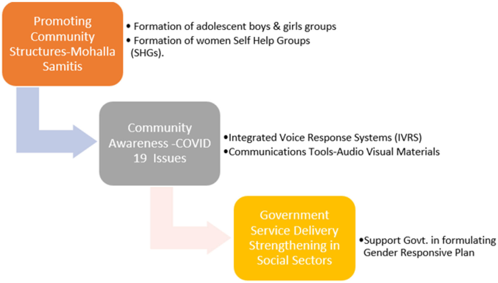
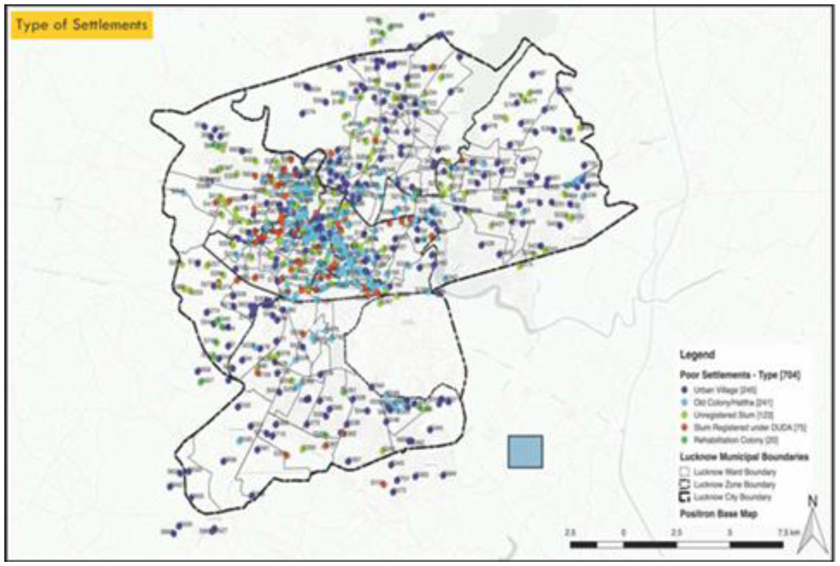
The SAMBHAV (Synchronized Action for Marginalized to Improve Behaviors and Vulnerabilities) initiative was launched between June 2020 to December 2020 by collaborating with the Uttar Pradesh state government, UNICEF and UNDP. The program intended to reach 6000 families in 30 UPS (Urban Poor settlements) of 13 city wards. These 30 UPS were divided into 5 clusters. The survey was conducted in 760 households, 397 taken from randomly selected 15 interventions and 363 households from 15 control UPS. This paper utilized data from a baseline assessment of gender and decision-making from a household survey conducted in the selected UPS during July 03–15, 2020. A sample size of 360 completed interviews was calculated for intervention and control areas to measure changes attributable to the SAMBHAV intervention in the behaviours and service utilization (pre- and post-intervention).
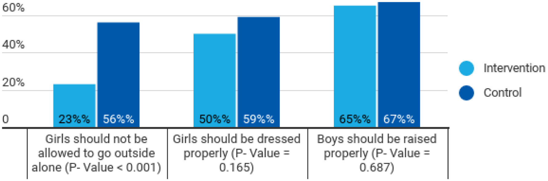
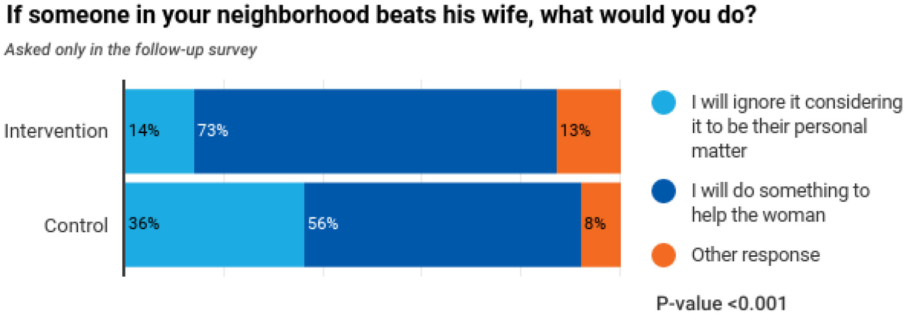
The data analysis showed a significant difference (p-value < 0.001) between respondents regarding women's freedom to move alone in the control and intervention area. It also reflected a significant difference between control and intervention areas as the respondents in the intervention area chose to work for the cause of gender-based violence.
The SAMBHAV initiative brought an intersectional lens to gender issues. The community volunteers were trained to approach issues based on gender-based violence with the local public, and various conferences and meetings were organized to sensitize the community. The initiative's overall impact was that it built momentum around the issue of applying the concept of intersectionality for gender issues and building resilience in the community. There is still a need to bring multi-layered and more aggressive approaches to reduce the prevalence of gender-based violence in the community.
Citation: Fnu Kajal, Ram Manohar Mishra, Amit Mehrotra, Vijay Kumar Chattu. Pandemic within a pandemic! Policy Implications of community-based Interventions to mitigate violence against women during COVID-19 in Urban Slums of Lucknow, India[J]. AIMS Public Health, 2023, 10(2): 297-309. doi: 10.3934/publichealth.2023022
The COVID-19 pandemic has brought an unprecedented adverse impact on women's health. Evidence from the literature suggests that violence against women has increased multifold. Gender-based violence in urban slums has worsened due to a lack of water and sanitation services, overcrowding, deteriorating conditions and a lack of institutional frameworks to address gender inequities.
The SAMBHAV (Synchronized Action for Marginalized to Improve Behaviors and Vulnerabilities) initiative was launched between June 2020 to December 2020 by collaborating with the Uttar Pradesh state government, UNICEF and UNDP. The program intended to reach 6000 families in 30 UPS (Urban Poor settlements) of 13 city wards. These 30 UPS were divided into 5 clusters. The survey was conducted in 760 households, 397 taken from randomly selected 15 interventions and 363 households from 15 control UPS. This paper utilized data from a baseline assessment of gender and decision-making from a household survey conducted in the selected UPS during July 03–15, 2020. A sample size of 360 completed interviews was calculated for intervention and control areas to measure changes attributable to the SAMBHAV intervention in the behaviours and service utilization (pre- and post-intervention).
The data analysis showed a significant difference (p-value < 0.001) between respondents regarding women's freedom to move alone in the control and intervention area. It also reflected a significant difference between control and intervention areas as the respondents in the intervention area chose to work for the cause of gender-based violence.
The SAMBHAV initiative brought an intersectional lens to gender issues. The community volunteers were trained to approach issues based on gender-based violence with the local public, and various conferences and meetings were organized to sensitize the community. The initiative's overall impact was that it built momentum around the issue of applying the concept of intersectionality for gender issues and building resilience in the community. There is still a need to bring multi-layered and more aggressive approaches to reduce the prevalence of gender-based violence in the community.

| [1] | Ministry of Home AffairsCensus of India Website: Office of the Registrar General & Census Commissioner, India (2011). Available from: https://censusindia.gov.in/census.website/data/HH2011. |
| [2] | UN Habitat, Slums: Some Definitions, State of the World's Cities. Available from: https://unhabitat.org/state-of-the-worlds-cities-20062007. |
| [3] | Ministry of Home Affairs G of ICensus of India Website: SRS Statistical Report (2011). Available from: https://censusindia.gov.in/nada/index.php/catalog/42684. |
| [4] |
Bailey RK Intimate Partner Violence: An Evidence-Based Approach (2021). https://doi.org/10.1007/978-3-030-55864-2 
|
| [5] |
Edwards KM (2015) Intimate Partner Violence and the Rural–Urban–Suburban Divide: Myth or Reality? A Critical Review of the Literature. Trauma Violence Abuse 16: 359-373. https://doi.org/10.1177/1524838014557289
|
| [6] |
Yakubovich AR, Heron J, Feder G, et al. (2020) Long-term Exposure to Neighborhood Deprivation and Intimate Partner Violence among Women: A UK Birth Cohort Study. Epidemiology 31: 272-281. https://doi.org/10.1097/EDE.0000000000001144
|
| [7] |
Jesmin SS (2017) Social Determinants of Married Women's Attitudinal Acceptance of Intimate Partner Violence. J Interpers Violence 32: 3226-3244. https://doi.org/10.1177/0886260515597436
|
| [8] |
Chakraborty D (2021) The “living dead” within “death-worlds”: Gender crisis and covid-19 in India. Gend Work Organ 28: 330-339. https://doi.org/10.1111/gwao.12585
|
| [9] | International Institute for Population SciencesNational Family Health Survey (NFHS-4) 2015–16 India (2017). Available from: http://rchiips.org/NFHS/NFHS-4Reports/India.pdf. |
| [10] | UN WomenViolence Against Women and Women's Economic Empowerment (2017). Available from: https://asiapacific.unwomen.org/en/news-and-events/stories/2017/10/addressing-violence-against-women-essential-to-economic-empowerment. |
| [11] |
Gaikwad V, Rao DH (2014) A cross-sectional study of domestic violence perpetrated by intimate partner against married women in the reproductive age group in an urban slum area in Mumbai. Indian J Public Heal Res Dev 5: 49-54. https://doi.org/10.5958/j.0976-5506.5.1.013
|
| [12] |
Begum S, Donta B, Nair S, et al. (2015) Socio-demographic factors associated with domestic violence in urban slums, Mumbai, Maharashtra, India. Indian J Med Res 141: 783-788. https://doi.org/10.4103/0971-5916.160701
|
| [13] |
Maji S, Bansod S, Singh T (2021) Domestic violence during COVID-19 pandemic: The case for Indian women. J Community Appl Soc Psychol 32: 374-381. https://doi.org/10.1002/casp.2501
|
| [14] |
Johnson K, Green L, Volpellier M, et al. (2020) The impact of COVID-19 on services for people affected by sexual and gender-based violence. Int J Gynecol Obstet 150: 285-287. https://doi.org/10.1002/ijgo.13285
|
| [15] |
Sharma P, Sharma S, Singh N (2020) COVID-19: Endangering women's mental and reproductive health. Indian J Public Health 64: 251-252. https://doi.org/10.4103/ijph.IJPH_498_20
|
| [16] |
Usher K, Bradbury Jones C, Bhullar N, et al. (2021) COVID-19 and family violence: Is this a perfect storm?. Int J Ment Health Nurs 30: 1022-1032. https://doi.org/10.1111/inm.12876
|
| [17] | Government of India D portalPradhan Mantri Garib Kalyan Package (PMGKP) | National Portal of India (2021). Available from: https://www.india.gov.in/spotlight/pradhan-mantri-garib-kalyan-package-pmgkp. |
| [18] |
Surma SA, Hakim SS, Rahman Lushan MS (2021) Planning for Pandemic Resilience: COVID-19 experience from urban slums in Khulna, Bangladesh. J Urban Manag 10: 325-344. https://doi.org/10.1016/j.jum.2021.08.003
|
| [19] |
George CE, Inbaraj LR (2021) Re: George et al. High seroprevalence of COVID-19 infection in a large slum in South India; what does it tell us about managing a pandemic and beyond?. Epidemiol Infect 149: e152. https://doi.org/10.1017/S0950268821001382
|
| [20] | WHOResponding to intimate partner violence and sexual violence against women (2011). Available from: https://www.who.int/publications/i/item/WHO-RHR-13.10. |
| [21] | IndiaCensus.net, Lucknow Population 2021. Available from: https://www.indiacensus.net/district/lucknow. |
| [22] | World Health Organization (WHO)Violence against women (2021). Available from: https://www.who.int/news-room/fact-sheets/detail/violence-against-women. |
| [23] |
Krishnakumar A, Verma S (2021) Understanding domestic violence in India during COVID-19: a routine activity approach. Asian J Criminol 16: 19-35. https://doi.org/10.1007/s11417-020-09340-1
|
| [24] |
Onditi F, Obimbo M, Muchina SK, et al. (2020) Modeling a pandemic (COVID-19) management strategy for urban slums using social geometry framework. Eur J Dev Res 32: 1450-1475. https://doi.org/10.1057/s41287-020-00317-5
|
| [25] |
Ryan NE, El Ayadi AM (2020) A call for a gender-responsive, intersectional approach to address COVID-19. Glob Public Health 15: 1404-1412. https://doi.org/10.1080/17441692.2020.1791214
|
Figures(4) / Tables(3)

Fnu Kajal, Ram Manohar Mishra, Amit Mehrotra, Vijay Kumar Chattu. Pandemic within a pandemic! Policy Implications of community-based Interventions to mitigate violence against women during COVID-19 in Urban Slums of Lucknow, India[J]. AIMS Public Health, 2023, 10(2): 297-309. doi: 10.3934/publichealth.2023022


 DownLoad: