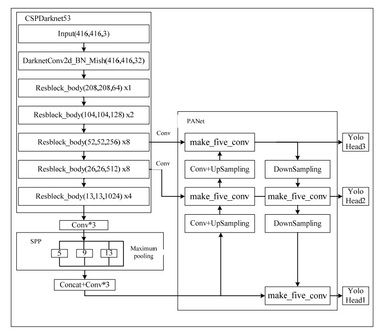
Aiming at the problem that the model of YOLOv4 algorithm has too many parameters and the detection effect of small targets is poor, this paper proposes an improved helmet fitting detection model based on YOLOv4 algorithm. Firstly, this model improves the detection accuracy of small targets by adding multi-scale prediction and improving the structure of PANet network. Then, the improved depth-separable convolution was used to replace the standard 3 × 3 convolution, which greatly reduced the model parameters without reducing the detection ability of the model. Finally, the k_means clustering algorithm is used to optimize the prior box. The model was tested on the self-made helmet dataset helmet_dataset. Experimental results show that compared with the safety helmet detection model based on Faster RCNN algorithm, the improved YOLOv4 algorithm has faster detection speed, higher detection accuracy and smaller number of model parameters. Compared with the original YOLOv4 model, the mAP of the improved YOLOv4 algorithm is increased by 0.49%, reaching 93.05%. The number of model parameters was reduced by about 58%, to about 105 MB. The model reasoning speed is 35 FPS. The improved YOLOv4 algorithm can meet the requirements of helmet wearing detection in multiple scenarios.
Citation: Haoyang Yu, Ye Tao, Wenhua Cui, Bing Liu, Tianwei Shi. Research on application of helmet wearing detection improved by YOLOv4 algorithm[J]. Mathematical Biosciences and Engineering, 2023, 20(5): 8685-8707. doi: 10.3934/mbe.2023381
Aiming at the problem that the model of YOLOv4 algorithm has too many parameters and the detection effect of small targets is poor, this paper proposes an improved helmet fitting detection model based on YOLOv4 algorithm. Firstly, this model improves the detection accuracy of small targets by adding multi-scale prediction and improving the structure of PANet network. Then, the improved depth-separable convolution was used to replace the standard 3 × 3 convolution, which greatly reduced the model parameters without reducing the detection ability of the model. Finally, the k_means clustering algorithm is used to optimize the prior box. The model was tested on the self-made helmet dataset helmet_dataset. Experimental results show that compared with the safety helmet detection model based on Faster RCNN algorithm, the improved YOLOv4 algorithm has faster detection speed, higher detection accuracy and smaller number of model parameters. Compared with the original YOLOv4 model, the mAP of the improved YOLOv4 algorithm is increased by 0.49%, reaching 93.05%. The number of model parameters was reduced by about 58%, to about 105 MB. The model reasoning speed is 35 FPS. The improved YOLOv4 algorithm can meet the requirements of helmet wearing detection in multiple scenarios.

| [1] |
H. Fan, Application of machine vision technology in Industrial inspection, Digital Commun. World, 12 (2020), 156–157. https://doi.org/10.3969/J.ISSN.1672-7274.2020.12.068 doi: 10.3969/J.ISSN.1672-7274.2020.12.068

|
| [2] |
D. G. Lowe, Distinctive image features from scaleinvariant keypoints, Int. J. Comput. Vision, 60 (2004), 91–110. https://doi.org/10.1023/B:VISI.0000029664.99615.94 doi: 10.1023/B:VISI.0000029664.99615.94
|
| [3] | N. Dalal, B. Triggs, Histograms of oriented gradients for human detection, in 2005 IEEE Computer Society Conference on Computer Vision and Pattern Recognition (CVPR'05), (2005), 886–893. https://doi.org/10.1109/CVPR.2005.177 |
| [4] |
J. Canny, A computational approch to edge detection, IEEE Trans. Pattern Anal. Mach. Intell, 8 (1986), 679–698. https://doi.org/10.1109/TPAMI.1986.4767851 doi: 10.1109/TPAMI.1986.4767851
|
| [5] | Q. Li, A Research and Implementation of Safety-helmetVideo Detection System Based onHuman Body Recognition, University of Electronic Science and Technology in Chengdu, M. S. thesis, 2017. |
| [6] |
S. Xu, Y. Wang, Y. Gu, N. Li, L. Zhuang, L. Shi, Safety helmet wearing detection study based on improved Faster RCNN, Appl. Res. Comput., 37 (2020), 267–271. https://doi.org/10.19734/j.issn.1001-3695.2018.07.0667 doi: 10.19734/j.issn.1001-3695.2018.07.0667
|
| [7] |
D. Wu, H. Wang, J Li, Safety helmet detection and identification based on improved faster RCNN, Inf. Technol. Informatization, 1 (2020), 17–20. https://doi.org/10.3969/j.issn.1672-9528.2020.01.003 doi: 10.3969/j.issn.1672-9528.2020.01.003
|
| [8] |
H. Wang, Z.Hu, Y. Guo, Z. Yang, F. Zhou, P. Xu, A real-time safety helmet wearing detection approach based on CSYOLOv3, Appl. Sci., 10 (2020), 6732. https://doi.org/10.3390/app10196732 doi: 10.3390/app10196732
|
| [9] | Y. Zhang, K. Wu, K. Gao, X. Yang, Helmet detection based on modified yolov3, Comput. Simul., 38 (2021), 5–10. |
| [10] | Y. Gu, Y. Wang, L. Shi, N. Li, L. Zhang, S. Xu, Automatic detection of safety helmet wearing based on head region location, IET Image Process., 15 (2021), 2441–2453. https://doi.org/10.1049/ipr2.12231 |
| [11] | Y. Cong, X. He, H. Zhu, X. Zhu, Helmet Monitoring System Based on Improved Yolov4-Tiny Network, Electron. Technol. Software Eng., 19 (2021), 121–124. |
| [12] | F. Wang, L. Chen, L. Jiao, Research on the algorithm of helmet detection based on SSD-MobileNet, Inf. Res., 3 (2020), 34–39. |
| [13] | A. G. Howard, M. Zhu, B. Chen, D. Kalenichenko, W. Wang, T. Weyand, et al., MobileNets: Efficient convolutional neural networks for mobile vision applications, 2017. Available from: https://www.semanticscholar.org/reader/3647d6d0f151dc05626449ee09cc7bce55be497e |
| [14] |
T. Xiao, L. Cai, K. Tang, X. Gao, C. Zhang, Improved SSD's Helmet wearing detection method, J. Sichuan Univ. Light Chem. Technol.: Nat. Sci. Ed., 33 (2020), 9–15. https://doi.org/10.11863/j.suse.2020.04.10 doi: 10.11863/j.suse.2020.04.10
|
| [15] | A. Howard, M. Sandler, G. Chu, W. Wang, L. Chen, M. Tan, et al, Searching for MobileNetV3, in 2019 IEEE/CVF International Conference on Computer Vision (ICCV), (2019), 1314–1324. https://doi.org/10.1109/ICCV.2019.00140 |


Figures(18) / Tables(6)

Haoyang Yu, Ye Tao, Wenhua Cui, Bing Liu, Tianwei Shi. Research on application of helmet wearing detection improved by YOLOv4 algorithm[J]. Mathematical Biosciences and Engineering, 2023, 20(5): 8685-8707. doi: 10.3934/mbe.2023381


 DownLoad: