|


Contact networks are heterogeneous. People with similar characteristics are more likely to interact, a phenomenon called assortative mixing or homophily. Empirical age-stratified social contact matrices have been derived by extensive survey work. We lack however similar empirical studies that provide social contact matrices for a population stratified by attributes beyond age, such as gender, sexual orientation, or ethnicity. Accounting for heterogeneities with respect to these attributes can have a profound effect on model dynamics. Here, we introduce a new method, which uses linear algebra and non-linear optimization, to expand a given contact matrix to populations stratified by binary attributes with a known level of homophily. Using a standard epidemiological model, we highlight the effect homophily can have on model dynamics, and conclude by briefly describing more complicated extensions. The available Python source code enables any modeler to account for the presence of homophily with respect to binary attributes in contact patterns, ultimately yielding more accurate predictive models.
Citation: Claus Kadelka. Projecting social contact matrices to populations stratified by binary attributes with known homophily[J]. Mathematical Biosciences and Engineering, 2023, 20(2): 3282-3300. doi: 10.3934/mbe.2023154
| [1] | Juan Pablo Aparicio, Carlos Castillo-Chávez . Mathematical modelling of tuberculosis epidemics. Mathematical Biosciences and Engineering, 2009, 6(2): 209-237. doi: 10.3934/mbe.2009.6.209 |
| [2] | Sara Y. Del Valle, J. M. Hyman, Nakul Chitnis . Mathematical models of contact patterns between age groups for predicting the spread of infectious diseases. Mathematical Biosciences and Engineering, 2013, 10(5&6): 1475-1497. doi: 10.3934/mbe.2013.10.1475 |
| [3] | Abdelkarim Lamghari, Dramane Sam Idris Kanté, Aissam Jebrane, Abdelilah Hakim . Modeling the impact of distancing measures on infectious disease spread: a case study of COVID-19 in the Moroccan population. Mathematical Biosciences and Engineering, 2024, 21(3): 4370-4396. doi: 10.3934/mbe.2024193 |
| [4] | Luis F. Gordillo, Stephen A. Marion, Priscilla E. Greenwood . The effect of patterns of infectiousness on epidemic size. Mathematical Biosciences and Engineering, 2008, 5(3): 429-435. doi: 10.3934/mbe.2008.5.429 |
| [5] | Suzanne M. O'Regan, John M. Drake . Finite mixture models of superspreading in epidemics. Mathematical Biosciences and Engineering, 2025, 22(5): 1081-1108. doi: 10.3934/mbe.2025039 |
| [6] | Maddalena Donà, Pieter Trapman . Possible counter-intuitive impact of local vaccine mandates for vaccine-preventable infectious diseases. Mathematical Biosciences and Engineering, 2024, 21(7): 6521-6538. doi: 10.3934/mbe.2024284 |
| [7] | Avery Meiksin . Using the SEIR model to constrain the role of contaminated fomites in spreading an epidemic: An application to COVID-19 in the UK. Mathematical Biosciences and Engineering, 2022, 19(4): 3564-3590. doi: 10.3934/mbe.2022164 |
| [8] | Cruz Vargas-De-León, Alberto d'Onofrio . Global stability of infectious disease models with contact rate as a function of prevalence index. Mathematical Biosciences and Engineering, 2017, 14(4): 1019-1033. doi: 10.3934/mbe.2017053 |
| [9] | Tong Zhang, Hiroshi Nishiura . COVID-19 cases with a contact history: A modeling study of contact history-stratified data in Japan. Mathematical Biosciences and Engineering, 2023, 20(2): 3661-3676. doi: 10.3934/mbe.2023171 |
| [10] | Nadia Loy, Andrea Tosin . A viral load-based model for epidemic spread on spatial networks. Mathematical Biosciences and Engineering, 2021, 18(5): 5635-5663. doi: 10.3934/mbe.2021285 |
Contact networks are heterogeneous. People with similar characteristics are more likely to interact, a phenomenon called assortative mixing or homophily. Empirical age-stratified social contact matrices have been derived by extensive survey work. We lack however similar empirical studies that provide social contact matrices for a population stratified by attributes beyond age, such as gender, sexual orientation, or ethnicity. Accounting for heterogeneities with respect to these attributes can have a profound effect on model dynamics. Here, we introduce a new method, which uses linear algebra and non-linear optimization, to expand a given contact matrix to populations stratified by binary attributes with a known level of homophily. Using a standard epidemiological model, we highlight the effect homophily can have on model dynamics, and conclude by briefly describing more complicated extensions. The available Python source code enables any modeler to account for the presence of homophily with respect to binary attributes in contact patterns, ultimately yielding more accurate predictive models.
Most social networks, e.g. physical interaction networks relevant to the spread of infectious diseases, exhibit assortative mixing, which describes the presence of more-than-expected interactions between network nodes with similar characteristics [1]. Assortative mixing is also known simply as assortativity, or as homophily in the case of social networks. Co-authorship networks in physics, biology and mathematics, film author collaboration networks, as well as Fortune 1000 company director networks are just some examples of social networks, which exhibit assortative mixing [1].
The seminal POLYMOD study supplied empirical evidence for the presence of strong age-assortative mixing in eight European countries [2]. Its main results are country-specific contact matrices, which describe the average number of daily contacts an individual of a certain age has with individuals of different ages, where the entire population is stratified into 5-year age bins (e.g., 0−4,5−9,…,80+). More recently, these contact matrices have been projected for 144 other countries including the United States, using surveys and demographic data [3].
Accurate infectious disease models must account for heterogeneous contact patterns in a population. During the COVID-19 pandemic, inclusion of realistic age-mixing patterns into infectious disease models has become increasingly popular, evident in the explosion of citations of [2,3]. While the available, empirically-grounded contact matrices account for homophily with respect to age, there are many other attributes (e.g., race/ethnicity, vaccine status, occupation, religion, education level or socio-economic status [4]) that are typically not included in epidemiological models. This is likely because there exist no empirical contact matrices that describe the assortative mixing with respect to attributes beyond age, partly because empirical studies that go beyond age present a great logistical challenge. For many of the aforementioned attributes however, we possess rough estimates of their homophily in a population. For example, it is well-established that there exists a strong level of ethnic homophily in the U.S. population [4,5].
In this manuscript, we describe a novel procedure that uses linear algebra and non-linear optimization techniques to infer contact matrices for populations stratified by age and additional attributes, for which estimates of their homophily exist. In this initial work, we require these attributes to be binary but extending to attributes with finitely-many values or categories should be straight-forward. In brief, we introduce a set of linear conditions a meaningful contact matrix should satisfy and show that there are typically infinitely many contact matrices that do so. To find the "optimal" contact matrix, we therefore define an objective function and pick the contact matrix that minimizes this function. User preference can inform the choice of objective function. Throughout the entire manuscript, we follow two simple examples and show that accounting for homophily can have a strong effect on model dynamics, i.e., how a pathogen spreads throughout a population.
Each individual in a population can be categorized using a multitude of attributes (e.g., age, ethnicity, education level). We can distinguish attributes by their range: some take on continuous values (e.g., age), while others are categorical (e.g., education level), discrete-valued or even binary (e.g., vaccinated against COVID-19 or not). As a whole, we can stratify a population based on a selection of attributes. In what follows, we assume all attributes take on only finitely many different values. This does not limit the usability of the developed methods, as binning can turn any continuous-valued attribute such as age into one with finitely-many choices, without losing substantial information if the number of bins is large. We begin with some basic definitions.
Definition 2.1. Let X1∈A1,…,Xd∈Ad be d attributes with 2≤|Ai|<∞. The (combined) attribute space A contains all possible d-tuples of attribute combinations. That is,
| A=A1×⋯×Ad. |
Given a population of size Ntotal, a (joint) distribution (or stratification) of that population based on the d attributes is a d-dimensional array N∈[0,∞)A with
| ∑i=(i1,…,id)∈ANi=Ntotal. |
Typically, Ntotal is a positive integer that describes the absolute number of individuals in the population. In some applications, it may however make more sense to set Ntotal=1 and consider Ni as the proportion of the total population. For the methods developed in this manuscript, how we interpret Ntotal does not matter.
Example 2.2. The age distribution, N=(N1,…,Nm), of a population split into m age groups is a non-negative (1-dimensional) vector of length m, which describes the number (or proportion) of individuals in each age group.
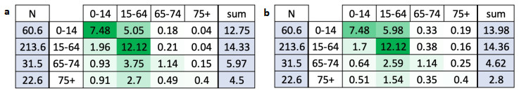
For the U.S. population and the four age groups defined as A={0−14,15−64,65−74,75+yearsofage}, the age distribution (absolute numbers in million) is N=(60.57,213.61,31.48,22.57), based on 2019 U.S. Census data [6].
To describe the rates of contacts between individuals with different attribute values, we introduce the concept of a contact matrix.
Definition 2.3. Given a population stratified across the combined attribute space A=A1×⋯×Ad, a contact function (also called contact matrix for reasons that become clear in the following remark) is a function
| C:A×A→[0,∞) |
that describes the average number of daily contacts an individual with attributes (i1,…,id)∈A has with individuals with attributes (j1,…,jd)∈A.
Remark 2.4. Given a combined d-dimensional attribute space A=A1×⋯×Ad, we can create an equivalent 1-dimensional attribute space whose attribute values are exactly the m:=∏|Ai| different combinations of attribute values in A. This motivates the use of the term "contact matrix" for the function C defined in Defintion 2.3, as it can be written as an m×m-matrix.
Remark 2.5. One can think of a distribution N of a population and a contact matrix C as two summary statistics of an undirected graph (i.e., a social interaction network) where the nodes (i.e., individuals) are labeled by the attribute values. Since the entry Cij in the contact matrix describes the average number of interactions (i.e., edges) connecting an individual with attribute i∈A with individuals with attribute j∈A, the total number of interactions between individuals with attributes i and j is given by NiCij whenever i≠j (and NiCii/2 otherwise). Due to the undirected nature of physical, real-world interactions, it is however also given by NjCji. A meaningful contact matrix representing physical interactions, relevant e.g. to describe the spread of an infectious disease, must therefore possess the following "symmetry" property.
Definition 2.6. (Reciprocity) Given a combined attribute space A and a corresponding distribution N of a population, a contact matrix C∈[0,∞)A×A is called reciprocal if for all i=(i1,…,id),j=(j1,…,jd)∈A,
| NiCij=NjCji. | (2.1) |
This property is often also referred to as symmetry; we avoid this term due to its ambiguity in matrix theory.
Example 2.7. An age-based contact matrix has been inferred for the United States [3] for age groups 0−4,5−9,…,75−79,80+. Using U.S. census data [6], this contact matrix can be condensed to the four age groups from Example 2.2 (Table 1a). The contact matrix is not reciprocal. To see this, we can compare e.g. the total number of reported daily contacts between 15−64 and 65−74 year olds. On the one hand, this number is
|
|
 DownLoad:
CSV
DownLoad:
CSV
| N2C23=213.6×106⋅0.21=44.9×10⁶. |
On the other hand, it is also given by
| N3C32=31.5×106⋅3.75=118.1×10⁶, |
which is not the same.
Empirical contact matrices stratified solely by age, such as those reported in the seminal POLYMOD study [2], are typically not reciprocal. This is because elderly people are generally more likely to report a short interaction as a contact. Extending the 1-dimensional transformation described in [7], an empirical contact matrix can however be easily transformed into a reciprocal one as follows.
Theorem 2.8. Given a combined attribute space A, a corresponding distribution N of a population, and a contact matrix C∈[0,∞)A×A, the transformed contact matrix ˜C defined by
| ˜Cij=NiCij+NjCji2Ni | (2.2) |
is reciprocal.
Proof. By design of the transformation, the total number of interactions between individuals with attributes i=(i1,…,id)∈A and j=(j1,…,jd)∈A is given by
| Ni˜Cij=NiCij+NjCji2=Nj˜Cji. |
Corollary 2.9. The total number of contacts in a population with reciprocal contact matrix C and distribution N over combined attribute space A is given by
| 12∑i∈A∑j∈ANiCij. |
Example 2.10. Using Theorem 2.8, we can transform the non-reciprocal U.S. contact matrix (Table 1a) into a reciprocal contact matrix (Table 1b).
We are now in a position to (i) define the homophily of a contact matrix with respect to a binary attribute and (ii) describe the problems arising when trying to project e.g. age-specific contact matrices to populations stratified by additional binary attributes with homophily. We look first at how homophily with respect to a binary attribute can be defined for an undirected labeled graph (e.g., a physical interaction network) and use the correspondence described in Remark 2.5 to define the homophily with respect to a binary attribute for a reciprocal contact matrix.
Definition 3.1. Given an undirected graph with nodes labeled by a binary attribute, we define the prevalence p∈[0,1] of the binary attribute as the proportion of nodes labeled true. We then distinguish between two types of edges: those connecting nodes with same and with opposite attribute values. As in [8], let ϕ∈[0,1] denote the proportion of edges connecting nodes with same attribute values.
In the case of complete segregation, we have ϕ=1 and the graph possesses two separate components. In the other extreme case of complete disassortativity, we have ϕ=0 and the graph is bipartite. Finally, in the absence of assortative mixing (i.e., no homophily), we have ϕ=E(ϕ) where
| E(ϕ)=p2+(1−p)2 | (3.1) |
as in [8]. Extending [8], we define the homophily h with respect to the binary attribute by comparing ϕ to its expected value,
| h(ϕ,p)={ϕ−E(ϕ)1−E(ϕ)∈[0,1]ifϕ≥E(ϕ),ϕ−E(ϕ)E(ϕ)∈[−1,0)ifϕ<E(ϕ). | (3.2) |
Example 3.2. If p=2/3 of individuals in a population are vaccinated against COVID-19, the expected number of interactions involving individuals with the same vaccination status is E(ϕ)=5/9. Thus if ϕ=5/9, there exists no homophily regarding vaccination status. If ϕ=7/9, the population exhibits 50% homophily. In the extreme case of ϕ=1, there exists 100% homophily (i.e., complete segregation), while the other extreme case of complete disassortativity with ϕ=0 corresponds to a homophily of −100% (or 100% heterophily).
Definition 3.3. Given a combined attribute space A=A1×⋯×Ad, a corresponding distribution N of a population and a contact matrix C∈[0,∞)A×A, we define the reduced attribute space without the kth attribute as
| A−k=A1×⋯×Ak−1×Ak+1×⋯×Ad. |
The reduced distribution without the kth attribute is a (d−1)-dimensional array N−k∈[0,∞)A−k such that for all i=(i1,…,ik−1,ik+1,…,id)∈A−k,
| N−ki=∑v∈AkNi1,…,ik−1,v,ik+1,…,id. |
Similarly, the reduced contact matrix without the kth attribute is a function C−k:A−k×A−k→[0,∞) such that for all i,j∈A−k,
| C−kij=∑v∈AkCi,(j1,…,jk−1,v,jk+1,…,jd). |
If the kth attribute is binary, assume w.l.o.g. Ak={0,1} and we define the attribute's prevalence in the population as the (d−1)-dimensional array P∈[0,1]A−k such that for all i=(i1,…,ik−1,ik+1,…,id)∈A−k,
| Pi=Ni1,…,ik−1,1,ik+1,…,idN−ki. |
If d=1, this definition corresponds exactly to the common language definition of "prevalence", used e.g. in Definition 3.1.
Definition 3.4. Let C∈[0,∞)A×A be a reciprocal contact matrix with A and N as before, and let the kth attribute be binary. Then, the homophily of the contact matrix with respect to the binary attribute can be defined by comparing the proportion of interactions between individuals with same attribute values, which is given by
| ϕ(C,N)=(∑i∈A∑j∈Ajk=ikNiCij)/(∑i∈A∑j∈ANiCij), | (3.3) |
to its expected number, E(ϕ), which can be computed from the prevalence P of the binary attribute, as follows.
W.l.o.g. assume that k=d and Ad={0,1}, i.e., the last attribute is binary, so that we can write (i,v) to denote (i1,…,id−1,v) for any i∈A−d and v∈Ad. In the absence of homophily, the binary attribute does not affect mixing patterns. For a given C, therefore, we can define a reciprocal contact matrix without homophily, denoted C0, by distributing according to the prevalence P the aggregated contacts in the reduced contact matrix. That is, for i,j∈A−d and v∈Ad, we have
| C0(i,v),(j,1)=PjC−kij,C0(i,v),(j,0)=(1−Pj)C−kij. | (3.4) |
By design, we now have
| E(ϕ)=ϕ(C0,N), |
and homophily is defined as in Equation 3.2,
| h(C,N)={ϕ(C,N)−E(ϕ)1−E(ϕ)∈[0,1]ifϕ(C,N)≥E(ϕ),ϕ(C,N)−E(ϕ)E(ϕ)∈[−1,0)ifϕ(C,N)≤E(ϕ). | (3.5) |
Remark 3.5. Similar to the definition of the non-homophilic contact matrix C0, we can define a contact matrix Ch that has homophily h∈(0,1] with respect to the dth binary attribute, by moving a proportion h of all contacts between opposite-valued individuals to equal-valued individuals. With Equation 3.4, that is for i,j∈A−d and v∈Ad={0,1},
| Ch(i,v),(j,v)=C0(i,v),(j,v)+hC0(i,v),(j,1−v)=(Pj,v+hPj,1−v)C−dij,Ch(i,v),(j,1−v)=(1−h)C0(i,v),(j,1−v)=(1−h)Pj,1−vC−dij, | (3.6) |
where
| Pj,v={Pjifv=1,1−Pjifv=0. | (3.7) |
While Ch has homophily h by definition, it is only reciprocal in special cases. To see this, consider e.g. (i,1),(j,1)∈A. Reciprocity implies
| N(i,1)Ch(i,1),(j,1)=N(j,1)Ch(j,1),(i,1)⟺PiN−di(Pj+h(1−Pj))C−dij=PjN−dj(Pi+h(1−Pi))C−dji, |
which due to the reciprocity of C is equivalent to
| Pi(Pj+h(1−Pj))=Pj(Pi+h(1−Pi))⟺(Pi−Pj)h=0. |
Ch is therefore only reciprocal if h=0 or if the prevalence is constant.
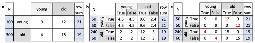
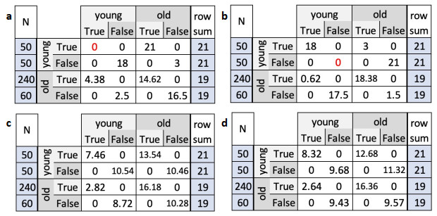
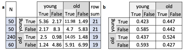
Example 3.6. Consider a population of size 400, which is stratified into (i) two age groups (e.g., young and old) with age distribution (100,300), and (ii) by an additional binary attribute with prevalence (0.5,0.8) across the age groups. Further assume an age-specific contact matrix (i.e., the reduced contact matrix without the second attribute, Definition 3.3) as in Table 2a. We can easily check that this contact matrix is reciprocal. Next, using the prevalence of the binary attribute, as described in Definition 3.4, we obtain a contact matrix C0 (Table 2b), which stratifies the population by both attributes and exhibits no homophily with respect to the binary attribute. This contact matrix is still reciprocal. As described in Remark 3.5, we can also define a contact matrix Ch with any given level of homophily for the binary attribute. In the extreme case of complete segregation (h=1), this would result in the contact matrix shown in Table 2c.
|
DownLoad:
CSV
Note that in both extended contact matrices, C0 and Ch, the total number of contacts an individual of a certain age has with individuals from each age group, and therefore also the total number of contacts (row sum), agrees with the basic age-age contact matrix, which is desirable. Ch is however not reciprocal (50⋅12≠240⋅4) because h≠0 and the prevalence of the binary attribute is not constant across age groups (Remark 3.5). Since reciprocity is a necessary condition for any physical contact matrix, relevant e.g. to study the spread of an infectious disease, this example motivates the need for a more elaborate approach.
In this section, we will develop methods to stratify a given contact matrix by an additional binary attribute with known prevalence and homophily. We start by describing a set of necessary conditions a meaningful extended contact matrix must satisfy. Any extended contact matrix that fails to satisfy some of these conditions is not suitable to accurately describe physical contacts and can, for example, not be used to study the spread of an infectious disease.
Definition 4.1. Given a combined attribute space A=A1×⋯×Ad, a corresponding distribution N of a population, a reciprocal contact matrix C∈[0,∞)A×A, and a binary attribute Xd+1 with known homophily h and prevalence P in the population, define N⋆ as the natural extension of the distribution (a function of N and P) over the extended attribute space A⋆=A×Ad+1,|Ad+1|=2 (to simplify notation, we frequently assume w.l.o.g. Ad+1={0,1}). An extended contact matrix C⋆∈[0,∞)A⋆×A⋆ is meaningful if it satisfies all of the following linear properties:
(a) Reciprocity: For all i,j∈A⋆,
| N⋆iC⋆ij=N⋆jC⋆ji |
(b) Same total contacts as in C: The total number of contacts of an individual should never depend on the value of the added binary attribute Xd+1. That is, for all i∈A,
| ∑j∈A⋆C⋆(i,0),j=∑j∈A⋆C⋆(i,1),j=∑j∈ACi,j. |
(c) Same contact patterns as in C: For all i,j∈A,
| ∑v∈Ad+1N⋆(i,v)Ni∑w∈Ad+1C⋆(i,v),(j,w)=Ci,j |
(d) Homophily: For the proportion ϕ of contacts between individuals with same binary attribute values (Equation 3.3) we have
| ϕ={E(ϕ)(1−h)+hifh≥0,E(ϕ)(1+h)ifh<0, |
where ϕ and E(ϕ) are computed as in Definition 3.4.
If h=1, we require ϕ=1. That is, for any i,j∈A,
| C⋆(i,0),(j,1)=C⋆(i,1),(j,0)=0. |
Likewise, if h=−1, we require ϕ=0. That is, for any i,j∈A,
| C⋆(i,0),(j,0)=C⋆(i,1),(j,1)=0. |
(e) If N⋆i=0 for some i∈A⋆, we can further assume C⋆ij=C⋆ji=0 for all j∈A⋆.
Remark 4.2. With m:=|A∗|, all conditions of Definition 4.1 can be written as a linear system of q equations
| Xc=y, | (4.1) |
where X is a q×m2 matrix, c is a vector of the m2 entries in the extended contact matrix C⋆ and y is a vector of the same dimension containing the "right-hand"-side of the linear equations.
Example 4.3. Given an age-specific contact matrix C with age groups young (y) and old (o) as in Table 2a and a binary attribute with prevalence (0.5,0.8) across the age groups and homophily h∈[0,1), an extended contact matrix C⋆ should satisfy:
(a) Reciprocity:
| 50 C⋆(y,1),(y,0)−50 C⋆(y,0),(y,1)=050 C⋆(y,1),(o,1)−240 C⋆(o,1),(y,1)=050 C⋆(y,1),(o,0)−60 C⋆(o,0),(y,1)=050 C⋆(y,0),(o,1)−240 C⋆(o,1),(y,0)=050 C⋆(y,0),(o,0)−60 C⋆(o,0),(y,0)=0240 C⋆(o,1),(o,0)−60 C⋆(o,0),(o,1)=0 |
(b) Same total contacts as in C:
| C⋆(y,1),(y,1)+C⋆(y,1),(y,0)+C⋆(y,1),(o,1)+C⋆(y,1),(o,0)=21C⋆(y,0),(y,1)+C⋆(y,0),(y,0)+C⋆(y,0),(o,1)+C⋆(y,0),(o,0)=21C⋆(o,1),(y,1)+C⋆(o,1),(y,0)+C⋆(o,1),(o,1)+C⋆(o,1),(o,0)=19C⋆(o,0),(y,1)+C⋆(o,0),(y,0)+C⋆(o,0),(o,1)+C⋆(o,0),(o,0)=19 |
(c) Same contact patterns as in C:
| 0.5 C⋆(y,1),(y,1)+0.5 C⋆(y,1),(y,0)+0.5 C⋆(y,0),(y,1)+0.5 C⋆(y,0),(y,0)=90.5 C⋆(y,1),(o,1)+0.5 C⋆(y,1),(o,0)+0.5 C⋆(y,0),(o,1)+0.5 C⋆(y,0),(o,0)=120.8 C⋆(o,1),(y,1)+0.8 C⋆(o,1),(y,0)+0.2 C⋆(o,0),(y,1)+0.2 C⋆(o,0),(y,0)=40.8 C⋆(o,1),(o,1)+0.8 C⋆(o,1),(o,0)+0.2 C⋆(o,0),(o,1)+0.2 C⋆(o,0),(o,0)=15 |
(d) Homophily:
| 50 C⋆(y,1),(y,0)+50 C⋆(y,1),(o,0)+50 C⋆(y,0),(o,1)+240 C⋆(o,1),(o,0)=(1−h)1545, |
where the number of interactions between nodes with opposite attribute values 1545=1−E(ϕ)=1−ϕ(C0,N) is derived from the extended contact matrix C0 without homophily shown in Table 2b. Thus to find an extended contact matrix that satisfies all desirable properties from Definition 4.1, we solve an under-determined non-homogeneous system of 15 linear equations in 16 variables, Xc=y, where dimNulX=4. If h=1, we have C⋆(i,v),(j,1−v)=0 for all i,j∈{y,o} and v∈{0,1}. Here, the properties (a)-(d) yield a system of 11 equations in 8 variables, where dimNulX=1.
Lemma 4.4. Given C,N,A,P as in Definition 4.1, let C0 be defined as in Equation 3.4. That is, for i,j∈A,v∈Ad+1,
| C0(i,v),(j,1)=PjCij,C0(i,v),(j,0)=(1−Pj)Cij. | (4.2) |
Then, C0 written as a vector c0∈[0,∞)m2 is a non-negative solution of Equation 4.1 for homophily h=0.
Proof. We start by showing C0 is reciprocal. Let i,j∈A and v∈Ad+1≅{0,1}. Remember Pj=N⋆(j,1)/Nj and 1−Pj=N⋆(j,0)/Nj. From the reciprocity of C, it follows that
| N⋆(i,v)C0(i,v),(j,1)=N⋆(i,v)PjCij=N⋆(i,v)N⋆(j,1)CijNj=N⋆(i,v)N⋆(j,1)CjiNi=N⋆(j,1)CjiN⋆(i,v)Ni=N⋆(j,1)Cji{Piifv=1(1−Pi)ifv=0=N⋆(j,1)C0(j,1),(i,v). |
Equivalently, we can show N⋆(i,v)C0(i,v),(j,0)=N⋆(i,v)C0(j,0),(i,v), which proves the reciprocity of C0. Properties (b) and (c) from Definition 4.1 follow very similarly. Finally, by design (see Definition 3.4) C0 exhibits no homophily (i.e., ϕ=E(ϕ)), which means c0 in vector form solves Equation 4.1 for homophily h=0. Non-negativity of c0 follows directly from C≥0 and Pj∈[0,1].
It is not clear if there exists a non-negative solution of Equation 4.1 for every choice of homophily h∈[−1,1]. It is however easy to see that the range of homophily values for which such a solution exists must be an interval.
Theorem 4.5. Given C,N,A,P as in Definition 4.1, there exists hmin,hmax with −1≤hmin≤0≤hmax≤1 such that Equation 4.1 has a non-negative solution if and only if h∈[hmin,hmax].
Proof. Let c0≥0 be the solution of Equation 4.1 for homophily 0 from Lemma 4.4. Further, assume ch is a non-negative solution to Equation 4.1 for homophily h∈(0,1]. Let α∈[0,1]. We show that the convex combination cα=αch+(1−α)c0 is a non-negative solution of Equation 4.1 for homophily αh. Let C0,Ch, and Cα denote the contact matrices corresponding to c0, ch, and cα, respectively.
(a) Reciprocity of Cα follows directly from the reciprocity of C0 and Ch: For all i,j∈A⋆,
| N⋆iCαij=αN⋆iChij+(1−α)N⋆iC0ij=αN⋆jChji+(1−α)N⋆jC0ji=N⋆jCαji. |
(b)-(c) Using the convex definition of Cα, it is similarly straight-forward to show that Cα contains the same total contacts and same contact patterns as the original contact matrix C (and as C0 and Ch).
(d) Let E:=E(ϕ). We know ϕ(C0,N)=E and ϕ(Ch,N)=h(1−E)+E. Due to the linear definition of ϕ (Equation 3.3), we have
| ϕ(Cα,N)=αϕ(Ch,N)+(1−α)ϕ(C0,N)=αh(1−E)+αE+(1−α)E=αh(1−E)+E, |
and therefore, with Equation 3.5, the homophily of Cα is
| h(Cα,N)=αh(1−E)+E−E1−E=αh. |
Non-negativity of Cα follows directly from Ch,C0≥0. Equivalently, one can show that cα is a non-negative solution of Equation 4.1 for homophily αh given we have a solution ch≥0 for h∈[−1,0).
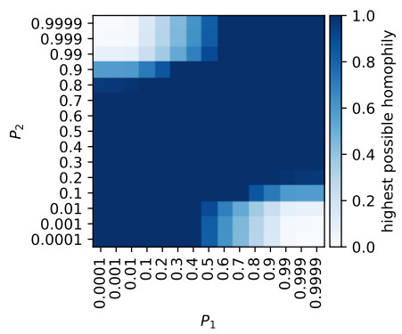
Example 4.6. Given C and N as in Table 2a, we have hmax=1 for most choices for the prevalence P=(P1,P2) of the added binary attribute (Figure 1). Only when P is very unbalanced, do we have hmax<1. Moreover, P2 is more important than P1 in determining if there exists a non-negative solution of Equation 4.1 for homophily h=1. This is likely because in this example old people outnumber young people, i.e., N2>N1, meaning an imbalance in the attribute distribution of the old people weighs more heavily.
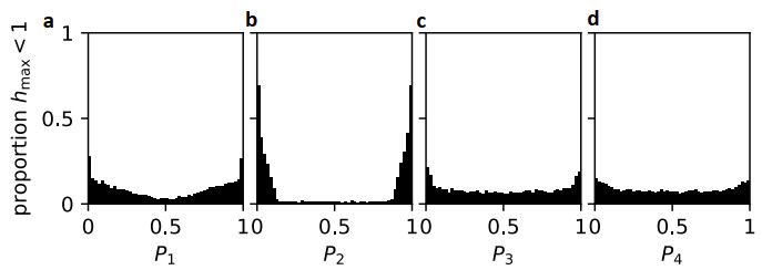
Example 4.7. If we stratify the U.S. population with age groups 0−14,15−64,65−74,75+ (and age distribution N and reciprocal contact matrix C as in Table 1b) by an additional binary attribute with prevalence P=(P1,P2,P3,P4), we can find a non-negative solution of Equation 4.1 for homophily h=1 for almost all choices of P. We generated 105 random prevalence vectors P∼U(0,1)4 and recorded whether we were able to obtain a solution c1≥0. Binning by Pi,i=1,…,4 confirms the observation made in the previous example that to ensure hmax=1, we primarily require a non-extreme prevalence for the age group with the largest population share, i.e., 15−64 year olds (with prevalence P2) in this example (Figure 2).
Remark 4.8. Given C,N,A,P as in Definition 4.1, Theorem 4.5 proves the existence of a non-negative solution ch of Equation 4.1 (i.e., a contact matrix Ch, which satisfies all properties of Definition 4.1) for certain choices of homophily h∈[−1,1]. Ch≥0 is however normally not a unique solution. To find the "best" contact matrix C⋆∈[0,∞)A⋆×A⋆, we define an objective function g:[0,∞)A⋆×A⋆→R and solve the following optimization problem with linear equality constraints:
| C⋆=argminC∈[0,∞)A⋆×A⋆g(C)subjecttoXc=y, | (4.3) |
where c∈[0,∞)m2 with m=|A∗| is, as before, the contact matrix C written as a column vector. Rather than solving this problem, we can solve a related, smaller problem over the null space of X with basis {b1,…,br}, using the known solution ch to formulate linear inequality constraints:
| C⋆=ch+argminx∈Rrg(ch+r∑i=1xibi)subjecttoch+r∑i=1xibi≥0. | (4.4) |
Example 4.9. For C,N,P defined as in Example 3.6 and homophily h=1, the null space of X is one-dimensional. Therefore, there exist infinitely many contact matrices that satisfy all desirable properties from Definition 4.1. The two extreme cases are shown in Table 3a, b. While both contact matrices have the same age-age contact patters as in C, they achieve this in the most unbalanced way. For instance, to obtain an average of C11=9 contacts for young people with young people, both matrices assign 18 contacts to one group of the young people (those with attribute value True or False, respectively) and none to the other group. Any convex combination of these two contact matrices will be more balanced.
|
DownLoad:
CSV
This example suggests an objective function that minimizes the differences in age-age contact patterns between people with opposite attribute value. Using the Euclidean distance, we can define the following objective function.
Definition 4.10. Let A⋆=A×Ad+1 with Ad+1={0,1} be an extended attribute space as in Definition 4.1. We define an objective function g:[0,∞)A⋆×A⋆→R that measures the balance in age-age contact patterns by
| g(C)=∑i∈A∑j∈A(C(i,1),(j,1)+C(i,1),(j,0)−C(i,0),(j,1)−C(i,0),(j,0))2. | (4.5) |
Example 4.11. The contact matrix shown in Table 3c minimizes g defined as in Equation 4.5. An alternative would be to define the least-squares solution (i.e., the contact matrix C that minimizes ||Xc−y|| from Equation 4.1) as optimal. This would result in the contact matrix shown in Table 3d.
When perfect segregation (h=1) is not desired but instead we require h∈(0,1), another objective function may be more useful. Instead of only looking at the overall homophily of a contact matrix with respect to a binary attribute, we can also define the specific homophily values for each split interaction.
Definition 4.12. Let A⋆=A×Ad+1 with Ad+1={0,1} be an extended attribute space as in Definition 4.1. Given a contact matrix C, we define the specific homophily of the contact patterns that an individual with attributes (i,v)∈A⋆ has with individuals with attributes j∈A by comparing the proportion of contacts between opposite-valued individuals with the expected proportion of such contacts, given prevalence P. That is,
| h(i,v),j(C,P)=1−C(i,v),(j,1−v)Pj,1−v(C(i,v),(j,v)+C(i,v),(j,1−v)), | (4.6) |
with Pj,1−v defined as in Equation 3.7.
Ideally, the specific homophily value for each split interaction should equal the overall homophily. As outlined in Remark 3.5 however, this is only possible if h=0 or if the prevalence is constant. Thus, we suggest as another objective to minimize the sum of the squared differences between the specific homophily values and the desired homophily.
Definition 4.13. Let A⋆=A×Ad+1 with Ad+1={0,1} be an extended attribute space as in Definition 4.1 and let h∈[0,1] be the desired level of (overall) homophily with respect to the added (d+1)th binary attribute. We define an objective function gh:[0,∞)A⋆×A⋆→R by setting
| gh(C)=∑i∈A∑j∈A∑v∈Ad+1(h(i,v),j(C,P)−h)2, | (4.7) |
with P denoting the prevalence.
Example 4.14. For C,N,P defined as in Example 3.6 and homophily h=0.5, the contact matrix shown in Table 4a minimizes gh, defined as in Equation 4.7. The specific homophily values, defined as in Equation 4.6, are shown in Table 4b. Due to the differences in the prevalence P=(0.5,0.8) of the binary attribute, a contact matrix where all specific homophily values equal h=0.5 is not possible, as it fails the reciprocity condition.
|
DownLoad:
CSV
Remark 4.15. By Remark 4.8, there are typically infinitely many contact matrices, which satisfy all properties of Definition 4.1. Which of these contact matrices we consider optimal depends on the specific choice of the objective function g. In Definitions 4.10 and 4.13, we describe two possible objective functions. For certain applications, other objective functions may yield more realistic contact matrices. Extreme contact matrices such as those shown in Table 3 a, b (see Example 4.9) are likely unrealistic and should be avoided as they can give rise to very different and unrealistic model dynamics.
In this section, we will compare a simple infectious disease model that only accounts for age-based mixing patterns with a more complicated model that accounts for an additional binary attribute with known homophily and prevalence. We show that disease dynamics may look quite different, especially if the homophily is high and the infection begins in one of the two groups.
Definition 5.1. A simple SIR (susceptible, infected, recovered) infectious disease model, in which the population is stratified into m groups (e.g., age groups or attribute-age groups) that accounts for assortative mixing is given by
| dSjdt=−λj(I)SjdIjdt=λj(I)Sj−rIjdRjdt=rIj |
for j=1,…,m. Here, r is the rate of recovery, the force of infection takes the form
| λj(I)=λj(I1,…,Im)=βm∑k=1CjkIk, |
β is the transmission rate and C∈[0,∞)m×m is the reciprocal contact matrix. As usual, we further assume that the population is closed with
| m∑j=1Sj+Ij+Rj=1. |
Example 5.2. To see the effect of homophily, consider C,N,P as in Example 3.6 and set β=0.05,r=0.1. Assume there exists no pre-existing immunity in the population, Rj(t=0)=0. Further, assume the disease starts in one sub-population, e.g.,
| Iyoung&True(t=0)=0.01 Nyoung&True, |
while for all other sub-populations j we have Ij(0)=0. A comparison of the disease dynamics for different levels of homophily reveals several phenomena (Figure 3):
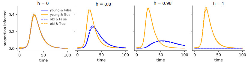
1. Even though initially only young people are infected, age does not matter much in the dynamics, likely because the contact matrix (Table 2a) exhibits very low homophily with respect to age.
2. The higher the homophily, the later and the lower the peak incidence appears among the individuals with an attribute value opposite to the one where the disease started. The presence of homophily thus introduces a delay mechanism. On the contrary, the higher the homophily, the earlier and higher the peak incidence appears among the sub-populations with the same attribute value as where the disease started. This is likely due to the requirement that the total number of contacts are constant, irrespective of the homophily. In the presence of high homophily, relatively more contacts happen between people with the same attribute value, leading to an increased spread of the disease within one group.
3. With increasing homophily (except for the extreme case of complete segregation, h=1), the time until the incidence falls below a certain threshold increases. This is likely because it takes more time for the disease to manifest itself among the sub-populations with attribute values opposite to the one where the disease started.
This example clearly shows the impact high levels of homophily can have on disease dynamics and that it can be important to account for the presence of homophily.
As outlined in Remark 2.5, contact matrices can also be used to generate undirected graphs. A homophilic contact matrix thus provides a way to obtain a more realistic interaction network, on which the spread of a pathogen through a community can be studied. The details of this application are however beyond the scope of this study.
Thus far, we have described how to expand a given contact matrix by a binary attribute with known prevalence and homophily. In this section, we will describe one of several possible extensions where in addition to the homophilic binary attribute the population is also split into several sub-populations with differential connectivity. This is, for example, needed to accurately model different contact levels due to occupation; e.g., people with public-facing jobs on average have a lot more contacts than people with office hours. Notice that in the absence of a homophilic binary attribute, a given contact matrix can be simply split into several sub-populations with differential connectivity by proportionately taking into account the relative sub-population sizes and their relative connectivity. We will now describe the linear conditions a meaningful contact matrix must satisfy in the more complicated case where we stratify the population by both a homophilic binary attribute and a binary attribute with differential connectivity.
Definition 6.1. Let A=A1×⋯×Ad be a combined attribute space, N a corresponding distribution of a population, C∈[0,∞)A×A a reciprocal contact matrix, and Xd+1 a binary attribute in Ad+1≅{0,1} with known homophily h as in Definition 4.1. Let Xd+2 be a finitely-valued attribute with values Ad+2 and known differential connectivity K∈(0,∞)|Ad+2|. That is, individuals with attribute value v2∈Ad+2 have Kv2/Kw2 times the number of contacts compared to individuals with attribute value w2∈Ad+2, assuming all other attributes in A×Ad+1 are the same. Further, let N⋆ be an extended distribution of the population corresponding to the extended attribute space A⋆=A×Ad+1×Ad+2.
An extended contact matrix C⋆∈[0,∞)A⋆×A⋆ is meaningful if it satisfies all of the following linear properties:
(a) Reciprocity (as in Definition 4.1): For all i,j∈A⋆,
| N⋆iC⋆ij=N⋆jC⋆ji |
(b) Same total contacts as in C:
(b1) The total number of contacts of an individual should never depend on the value of the added homophilic binary attribute Xd+1. That is, for all i∈A and all v2∈Ad+2,
| ∑j∈A⋆C⋆(i,0,v2),j=∑j∈A⋆C⋆(i,1,v2),j. |
(b2) Differential connectivity with respect to Xd+2 described by K. Fix ˉv∈Ad+2. Individuals with attribute v2∈Ad+2 possess Kv2/Kˉv times more contacts than individuals with attribute ˉv∈Ad+2 (and otherwise same characteristics). That is, for all i,j∈A and all v1∈Ad+1,
| KˉvC⋆(i,v1,v2),j=Kv2C⋆(i,v1,ˉv),j. |
(b3) The average total number of contacts of individuals with attribute (i,v1)∈A×Ad+1 is the same as in C. That is, for all i∈A, v1∈Ad+1,
| ∑v2∈Ad+2N⋆(i,v1,v2)∑w2∈Ad+2N⋆(i,v1,w2)∑j∈A⋆C⋆(i,v1,v2),j=∑j∈ACi,j. |
(c) Same contact patterns as in C (as in Definition 4.1): For all i,j∈A,
| ∑v1∈Ad+1∑v2∈Ad+2N⋆(i,v1,v2)Ni∑w1∈Ad+1∑w2∈Ad+2C⋆(i,v1,v2),(j,w1,w2)=Ci,j |
(d) Homophily (as in Definition 4.1): For the proportion ϕ of contacts between individuals with same binary attribute values (Equation 3.3) we have
| ϕ={E(ϕ)(1−h)+hifh≥0,E(ϕ)(1+h)ifh<0, |
where ϕ and E(ϕ) are computed as in Definition 3.4.
If h=1, we require ϕ=1. That is, for any i,j∈A and any v2,w2∈Ad+2,
| C⋆(i,0,v2),(j,1,w2)=C⋆(i,1,v2),(j,0,w2)=0. |
Likewise, if h=−1, we require ϕ=0. That is, for any i,j∈A and any v2,w2∈Ad+2,
| C⋆(i,0,v2),(j,0,w2)=C⋆(i,1,v2),(j,1,w2)=0. |
(e) If N⋆i=0 for some i∈A⋆, we can further assume (as in Definition 4.1) C⋆ij=C⋆ji=0 for all j∈A⋆.
Remark 6.2. To find the "best" meaningful extended contact matrix, one solves the same non-linear optimization problem as outlined in Section 4.
Remark 6.3. Definition 6.1 also includes all linear conditions needed to find a meaningful contact matrix extended by a binary homophilic attribute, where the two attribute values have differential connectivity. Simply set Ad+1=Ad+2≅{0,1} and use an extended distribution N⋆∈[0,∞)A⋆ with N⋆(i,v1,v2)=0 whenever v1≠v2.
The current COVID-19 pandemic has revealed the importance of accurate epidemic forecasting models. One key element of these models is a contact matrix that describes the rates of mixing between different sub-populations. Age constitutes the primary attribute used to stratify populations. This is partly because age, especially for COVID-19 with its disproportionate burden on older individuals, is an important variable but also partly because most empirical work on contact matrices focuses primarily on age. This study introduces new methodology enabling modelers to expand contact matrices using binary attributes for which the prevalence and the level of homophily in a population is known or can be estimated. We showed that the disease dynamics can be very different when homophily is included in a model. A more elaborate, recent model uses this new methodology and shows that accounting for homophily with respect to ethnicity is important when designing optimal vaccine roll-out strategies [9].
This manuscript leaves several questions unanswered. First, we only consider binary attributes. This means any non-binary attributes need to be binarized, which may not always be feasible or desirable. An extension to non-binary attributes should be straight-forward and ideas from [10] should prove useful in this effort. One possible difficulty, however, is that homophily can no longer be described by a single value, but requires (m2) variables where m is the number of attribute values. Finally, we presented only a simple, simulation-based application to show the effect of homophily on disease dynamics. Related theoretical considerations, such as investigating the effect of homophily on the effective reproductive number using next-generation matrices as in [11], should provide fruitful avenues for future research.
The author thanks Audrey McCombs for critical comments on the manuscript.
All relevant code is available at GitHub: https://github.com/ckadelka/HomophilicContactMatrices.
The author declares there is no conflict of interest.
| [1] |
M. E. Newman, Mixing patterns in networks, Phys. Rev. E, 67 (2003), 026126. https://doi.org/10.1103/PhysRevE.67.026126 doi: 10.1103/PhysRevE.67.026126

|
| [2] |
J. Mossong, N. Hens, M. Jit, P. Beutels, K. Auranen, R. Mikolajczyk, et al., Social contacts and mixing patterns relevant to the spread of infectious diseases, PLoS Med., 5 (2008), e74. https://doi.org/10.1371/journal.pmed.0050074 doi: 10.1371/journal.pmed.0050074
|
| [3] |
K. Prem, A. R. Cook, M. Jit, Projecting social contact matrices in 152 countries using contact surveys and demographic data, PLoS Comput. Biol., 13 (2017), e1005697. https://doi.org/10.1371/journal.pcbi.1005697 doi: 10.1371/journal.pcbi.1005697
|
| [4] |
M. McPherson, L. Smith-Lovin, J. M. Cook, Birds of a feather: Homophily in social networks, Ann. Rev. Sociol., 27 (2001), 415–444. https://doi.org/10.1146/annurev.soc.27.1.415 doi: 10.1146/annurev.soc.27.1.415
|
| [5] |
K. A. Mollica, B. Gray, L. K. Trevino, Racial homophily and its persistence in newcomers' social networks, Organiz. Sci., 14 (2003), 123–136. https://doi.org/10.1287/orsc.14.2.123.14994 doi: 10.1287/orsc.14.2.123.14994
|
| [6] | U.S. Census Bureau, American community survey 1-year estimates, 2019. Data retrieved from https://data.census.gov/cedsci/table?q=age&tid=ACSST1Y2019.S0101&hidePreview=false |
| [7] |
S. Funk, J. K. Knapp, E. Lebo, S. E. Reef, A. J. Dabbagh, K. Kretsinger, et al., Combining serological and contact data to derive target immunity levels for achieving and maintaining measles elimination, BMC Med., 17 (2019), 1–12. https://doi.org/10.1186/s12916-019-1413-7 doi: 10.1186/s12916-019-1413-7
|
| [8] |
C. Kadelka, A. McCombs, Effect of homophily and correlation of beliefs on COVID-19 and general infectious disease outbreaks, PloS One, 16 (2021), e0260973. https://doi.org/10.1371/journal.pone.0260973 doi: 10.1371/journal.pone.0260973
|
| [9] |
C. Kadelka, M. R. Islam, A. McCombs, J. Alston, N. Morton, Ethnic homophily affects vaccine prioritization strategies, J. Theor. Biol., 555 (2022), 111295. https://doi.org/10.1016/j.jtbi.2022.111295 doi: 10.1016/j.jtbi.2022.111295
|
| [10] |
Z. Feng, A. N. Hill, P. J. Smith, J. W. Glasser, An elaboration of theory about preventing outbreaks in homogeneous populations to include heterogeneity or preferential mixing, J. Theor. Biol., 386 (2015), 177–187. https://doi.org/10.1016/j.jtbi.2015.09.006 doi: 10.1016/j.jtbi.2015.09.006
|
| [11] |
O. Diekmann, J. Heesterbeek, M. G. Roberts, The construction of next-generation matrices for compartmental epidemic models, J. Royal Soc. Interf., 7 (2010), 873–885. https://doi.org/10.1098/rsif.2009.0386 doi: 10.1098/rsif.2009.0386
|
| 1. | Zhijun Wu, Vincent Antonio Traag, Beyond six feet: The collective behavior of social distancing, 2024, 19, 1932-6203, e0293489, 10.1371/journal.pone.0293489 | |
| 2. | Vaibhava Srivastava, Drik Sarkar, Claus Kadelka, Model-informed optimal allocation of limited resources to mitigate infectious disease outbreaks in societies at war, 2024, 21, 1742-5689, 10.1098/rsif.2024.0575 | |
| 3. | Yaxu Zheng, Bo Zheng, Xiaohuan Gong, Hao Pan, Chenyan Jiang, Shenghua Mao, Sheng Lin, Bihong Jin, Dechuan Kong, Ye Yao, Genming Zhao, Huanyu Wu, Weibing Wang, Contact patterns between index patients and their close contacts and assessing risk for COVID-19 transmission during different exposure time windows: a large retrospective observational study of 450 770 close contacts in Shanghai, 2024, 2, 2753-4294, e000154, 10.1136/bmjph-2023-000154 | |
| 4. | Loukas Zachilas, Christos Benos, Modeling and Visualizing the Dynamic Spread of Epidemic Diseases—The COVID-19 Case, 2023, 4, 2673-9909, 1, 10.3390/appliedmath4010001 | |
| 5. | Gilberto González-Parra, Hana M. Dobrovolny, Editorial: Mathematical foundations in biological modelling and simulation, 2024, 21, 1551-0018, 7084, 10.3934/mbe.2024311 | |
| 6. | Gilberto González-Parra, Md Shahriar Mahmud, Claus Kadelka, Learning from the COVID-19 pandemic: A systematic review of mathematical vaccine prioritization models, 2024, 9, 24680427, 1057, 10.1016/j.idm.2024.05.005 | |
| 7. | Shuanger Li, Davorka Gulisija, Oana Carja, Roger Dimitri Kouyos, The evolutionary cost of homophily: Social stratification facilitates stable variant coexistence and increased rates of evolution in host-associated pathogens, 2024, 20, 1553-7358, e1012619, 10.1371/journal.pcbi.1012619 |
Figures(3) / Tables(4)

Claus Kadelka. Projecting social contact matrices to populations stratified by binary attributes with known homophily[J]. Mathematical Biosciences and Engineering, 2023, 20(2): 3282-3300. doi: 10.3934/mbe.2023154

|
|
DownLoad:
CSV
|
|
DownLoad:
CSV
|
|
DownLoad:
CSV
|
|
DownLoad:
CSV
