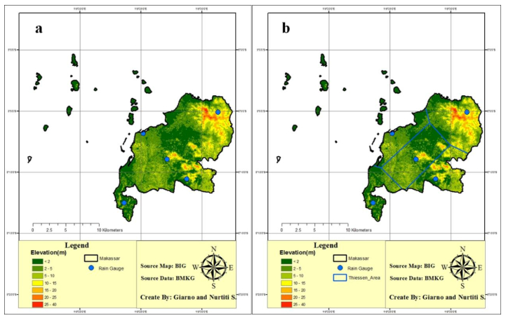
Improving the accuracy of rainfall forecasts is related to the number of rain gauges needed in an area, so determining the optimal number of rain gauges is very important. This study aimed to determine the best method for calculating the optimal number of rain gauges. Generally, the calculation of the optimal number of rain gauges using the coefficient of variation only takes into account the accumulation of rainfall at the station. The distance between the location and height of the rain gauge is not taken into account. The phenomenon of rain that occurs in the tropics is very dynamic, where one place compared to another tends to have different rain intensity and duration. In addition, the height and distance factors also greatly affect the measured rainfall. Therefore, it is very important to know the best method to calculate the optimal number of rain gauges needed in a particular area. This study implements 3 methods to determine the appropriate method to be used in determining the optimal rain gauge number for urban areas: namely, World Meteorological Organization (WMO) criteria, coefficient of variation, and Kagan-Rodda. In this study, rainfall data from 2010 to 2019 at 5 locations in Makassar were used in calculating the optimal number of rain gauges required. The results showed that the optimal number of rain gauges in Makassar as an urban area following the WMO recommendation was 9–18, where small islands around it are not considered. Another result obtained is that if the rainfall data for the Sudiang area, which is located at the coordinates (119.522° E, 5.085° S), is not included in the calculation, it will greatly reduce the accuracy in determining the optimal number of rain gauges in the Makassar area.
Citation: Nurtiti Sunusi, Giarno. Comparison of some schemes for determining the optimal number of rain gauges in a specific area: A case study in an urban area of South Sulawesi, Indonesia[J]. AIMS Environmental Science, 2022, 9(3): 260-276. doi: 10.3934/environsci.2022018
Improving the accuracy of rainfall forecasts is related to the number of rain gauges needed in an area, so determining the optimal number of rain gauges is very important. This study aimed to determine the best method for calculating the optimal number of rain gauges. Generally, the calculation of the optimal number of rain gauges using the coefficient of variation only takes into account the accumulation of rainfall at the station. The distance between the location and height of the rain gauge is not taken into account. The phenomenon of rain that occurs in the tropics is very dynamic, where one place compared to another tends to have different rain intensity and duration. In addition, the height and distance factors also greatly affect the measured rainfall. Therefore, it is very important to know the best method to calculate the optimal number of rain gauges needed in a particular area. This study implements 3 methods to determine the appropriate method to be used in determining the optimal rain gauge number for urban areas: namely, World Meteorological Organization (WMO) criteria, coefficient of variation, and Kagan-Rodda. In this study, rainfall data from 2010 to 2019 at 5 locations in Makassar were used in calculating the optimal number of rain gauges required. The results showed that the optimal number of rain gauges in Makassar as an urban area following the WMO recommendation was 9–18, where small islands around it are not considered. Another result obtained is that if the rainfall data for the Sudiang area, which is located at the coordinates (119.522° E, 5.085° S), is not included in the calculation, it will greatly reduce the accuracy in determining the optimal number of rain gauges in the Makassar area.

| [1] |
S. K. Adhikary, A. G. Yilmaz, N. Muttil (2015) Optimal design of rain gauge network in the Middle Yarra River catchment, Australia. Hydrol Process 29: 2582–2599. https://doi.org/10.1002/hyp.10389 doi: 10.1002/hyp.10389

|
| [2] | P. R. Ahuja (1960) Planning of precipitation network for water resources development in India. WMO flood control series 15: 106–112. |
| [3] | A. M. Al-Abadi, A. H. D. Al-Aboodi (2014) Optimum rain-gauges network design of some cities in Iraq. J Babylon Uni/Eng Sci 22: 946–958. |
| [4] |
R. D'Arrigo, R. Wilson (2008) Short Communication: El Niño and Indian Ocean influences on Indonesian drought: implications for forecasting rainfall and crop productivity. Int J Climatology 28: 611–616. https://doi.org/10.1002/joc.1654 doi: 10.1002/joc.1654
|
| [5] | J. D. Evans (1996) Straight forward statistics for the behavioral sciences, Brooks/Cole Pub Co Pacific Grove. |
| [6] |
Giarno, M. P. Hadi, S. Suprayogi, et al. (2018) Distribution of accuracy of TRMM daily rainfall in Makassar Strait. Forum Geografi 32: 38–52. https://doi.org/10.23917/forgeo.v32i1.5774 doi: 10.23917/forgeo.v32i1.5774
|
| [7] | Giarno, Muflihah, Mujahiddin (2001) Determination of optimal rain gauge on the coastal region use coefficient variation: Case study in Makassar. J Civil Eng Forum 7: 121–132. |
| [8] | P. Goovaerts (1997) Geostatistics for Natural Resources Evaluation. Oxford Univ Press, New York. |
| [9] |
M. Hanel, P. Máca (2014) Spatial variability and interdependence of rain event characteristics in the Czech Republic. Hydrol Process 28: 2929–2944. https://doi.org/10.1002/hyp.9845 doi: 10.1002/hyp.9845
|
| [10] |
D. Harisuseno, E. Suhartono, D. M. Cipta (2020) Rainfall streamflow relationship using stepwise method as a basis for rationalization of rain gauge network Density. Int J Recent Tech Eng 8: 2277–3878. https://doi.org/10.35940/ijrte.E6617.018520 doi: 10.35940/ijrte.E6617.018520
|
| [11] | R. L. Kagan (1972) Planning the spatial distribution of hydrometeorological stations to meet an error criterion. In: Casebook on Hydrological Network Design Practice, III-1, WMO Publication 324. |
| [12] |
A. K. Mishra, P. Coulibaly (2009) Developments in hydrometric network design: A review. Rev Geoph 47: 1–24. https://doi.org/10.1029/2007RG000243 doi: 10.1029/2007RG000243
|
| [13] | S. Karmakar, A. Rahman, S. M. Q. Hassan (2012) Variability of monsoon rainfall and its interstation correlation in Bangladesh. The J Noami 29: 33–54. |
| [14] | A. D. Patel, M. B. Dholakia, D. P. Patel, et al. (2016) Analysis of optimum number of rain Gauge in Shetrunji River Basin, Gujarat - India. Int J Sci Tech & Eng 2: 380–384. |
| [15] |
B. U. Ngene, J. C. Agunwamba, B. A. Nwachukwu (2018) The Challenges to Nigerian raingauge network improvement. Res J Env Earth Sci 7: 68–74. https://doi.org/10.19026/rjees.7.2205 doi: 10.19026/rjees.7.2205
|
| [16] |
M. Martono, T. Wardoyo (2017) Impacts of El Niño 2015 and the Indian Ocean Dipole 2016 on rainfall in the Pameungpeuk and Cilacap regions. Forum Geografi 31: 184–195. https://doi.org/10.23917/forgeo.v31i2.4170 doi: 10.23917/forgeo.v31i2.4170
|
| [17] | F. Y. Pramono, S. Suripin, W. Sulistya (2019) Rationalization of rain stations in the Ciliwung Cisadane river basin. Int J Eng Res Tech 12: 2957–2963. |
| [18] | Supari, F. Tangang, E. Salimun, et al. (2012) ENSO modulation of seasonal rainfall and extremes in Indonesia. Climate Dynamics 2012: 1–22. |
| [19] | H. M. Raghunath (2006) Hydrology: Principles, Analysis, and Design. New Age International Publishers, Second Edition. |
| [20] |
Z. Sen, Z. Habib (2001) Monthly spatial rainfall correlation functions and interpretations for Turkey. Hydrology Sciences Journal 46: 525–535. https://doi.org/10.1080/02626660109492848 doi: 10.1080/02626660109492848
|
| [21] | M. R. Shaghaghian, M. J. Abedini (2013) Rain gauge network design using coupled geostatistical and multivariate technique. Scientia Iranica 20: 259–269. |
| [22] |
H. B. Rycroft (1949) Random sampling of rainfall. J South African Forestry Assoc 18: 71–81. https://doi.org/10.1080/03759873.1949.9630653 doi: 10.1080/03759873.1949.9630653
|
| [23] | Akoglu, H., 2018, User's guide to correlation coefficients, Turkish Journal of Emergency Medicine, 18, 91–93 |
| [24] |
H. S. Lee (2015) General rainfall patterns in Indonesia and the potential impacts of local seas on rainfall intensity. Water 7: 1750-1768. https://doi.org/10.3390/w7041751 doi: 10.3390/w7041751
|
| [25] | WMO (1972) Casebook on hydrological network design practice. WMO, 324. |
| [26] | WMO (1994) Guide to hydrological practices: Data acquisition and processing, analysis, forecasting, and other applications. WMO, 168. |
| [27] |
F. A. Sneva, L. D. Calvin (1978) An improved Thiessen grid for eastern Oregon: An interstation correlation study determining the effect of the distance, bearing, and elevation between stations upon the precipitation correlation coefficient. Agricultural Meteorology 9: 471–483. https://doi.org/10.1016/0002-1571(78)90044-4 doi: 10.1016/0002-1571(78)90044-4
|
| [28] |
H. C. Yeh, Y. C. Chen, C. Wei, et al. (2011) Entropy and kriging approach to rainfall network design. Paddy Water Env 9: 343–355. https://doi.org/10.1007/s10333-010-0247-x doi: 10.1007/s10333-010-0247-x
|
| [29] |
N. Sunusi, E. T. Herdiani (2017) Modeling of extreme rainfall recurrence time by using point process models. J Env Sci Tech 10: 320–324. https://doi.org/10.3923/jest.2017.320.324 doi: 10.3923/jest.2017.320.324
|
| [30] |
V. Svoboda, P. Maca, M. Hanel, et al. (2015) Spatial correlation structure of monthly rainfall at a mesoscale region of north-eastern Bohemia. Theor Appl Climatol 121: 359–375. https://doi.org/10.1007/s00704-014-1241-9 doi: 10.1007/s00704-014-1241-9
|
| [31] |
R. Avanzato, F. Beritelli (2020) An innovative acoustic rain gauge based on convolutional neural networks. Information 11: 1–16. https://doi.org/10.3390/info11040183 doi: 10.3390/info11040183
|
| [32] |
R. Avanzato, F. Beritelli (2020) Hydrogeological risk management in smart cities: A new approach to rainfall classification based on LTE cell selection parameters. IEEE Access 8: 137161–137173. https://doi.org/10.1109/ACCESS.2020.3011375. doi: 10.1109/ACCESS.2020.3011375
|


Figures(3) / Tables(6)

Nurtiti Sunusi, Giarno. Comparison of some schemes for determining the optimal number of rain gauges in a specific area: A case study in an urban area of South Sulawesi, Indonesia[J]. AIMS Environmental Science, 2022, 9(3): 260-276. doi: 10.3934/environsci.2022018


 DownLoad: