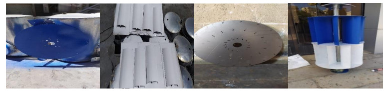
This is an experimental study that investigates the performance of a hybrid wind-solar street lighting system and its cost of energy. The site local design conditions of solar irradiation and wind velocity were employed in the design of the system components. HOMER software was also used to determine the Levelized Cost of Energy (LCOE) and energy performance indices, which provides an assessment of the system's economic feasibility. The hybrid power supply system comprised of an integrated two photovoltaic (PV) solar modules and a combined Banki-Darrieus wind turbines. The second PV module was used to extend the battery storage for longer runtime, and the Banki-Darrieus wind turbines were used also to boost the battery charge for times when there is wind but no sunshine, especially in winter and at night. The results indicated that the hybrid system proved to be operating successfully to supply power for a street LED light of 30 watts. A wind power of 113 W was reached for a maximum wind speed that was recorded in the year 2021 of 12.10 m/s. The efficiency of the combined Banki-Darrieus wind turbine is 56.64%. In addition, based on the HOMER optimization analysis of three scenarios, of which, using either a solar PV system or the combined wind turbines each alone, or using the hybrid wind-solar system. The software results showed that the hybrid wind-solar system is the most economically feasible case.
Citation: Nadwan Majeed Ali, Handri Ammari. Design of a hybrid wind-solar street lighting system to power LED lights on highway poles[J]. AIMS Energy, 2022, 10(2): 177-190. doi: 10.3934/energy.2022010
This is an experimental study that investigates the performance of a hybrid wind-solar street lighting system and its cost of energy. The site local design conditions of solar irradiation and wind velocity were employed in the design of the system components. HOMER software was also used to determine the Levelized Cost of Energy (LCOE) and energy performance indices, which provides an assessment of the system's economic feasibility. The hybrid power supply system comprised of an integrated two photovoltaic (PV) solar modules and a combined Banki-Darrieus wind turbines. The second PV module was used to extend the battery storage for longer runtime, and the Banki-Darrieus wind turbines were used also to boost the battery charge for times when there is wind but no sunshine, especially in winter and at night. The results indicated that the hybrid system proved to be operating successfully to supply power for a street LED light of 30 watts. A wind power of 113 W was reached for a maximum wind speed that was recorded in the year 2021 of 12.10 m/s. The efficiency of the combined Banki-Darrieus wind turbine is 56.64%. In addition, based on the HOMER optimization analysis of three scenarios, of which, using either a solar PV system or the combined wind turbines each alone, or using the hybrid wind-solar system. The software results showed that the hybrid wind-solar system is the most economically feasible case.

| [1] |
Khare V, Nema S, Baredar P (2016) Solar-wind hybrid renewable energy system: A review. Renew Sustain Energy Rev 58: 23–33. https://doi.org/10.1016/j.rser.2015.12.223 doi: 10.1016/j.rser.2015.12.223

|
| [2] |
Al-Tarawneh L, Alqatawneh A, Tahat A, et al. (2021) Evolution of optical networks: From legacy networks to next-generation networks. J Opt Commun 2020. https://doi.org/10.1515/joc-2020-0108 doi: 10.1515/joc-2020-0108
|
| [3] |
Mazzeo D, Herdem MS, Matera N, et al. (2021) Artificial intelligence application for the performance prediction of a clean energy community. Energy 232. https://doi.org/10.1016/j.energy.2021.120999 doi: 10.1016/j.energy.2021.120999
|
| [4] |
Elmorshedy MF, Elkadeem MR, Kotb KM, et al. (2021) Optimal design and energy management of an isolated fully renewable energy system integrating batteries and supercapacitors. Energy Convers Manage 245. https://doi.org/10.1016/j.enconman.2021.114584 doi: 10.1016/j.enconman.2021.114584
|
| [5] |
Mazzeo D, Matera N, de Luca P, et al. (2021) A literature review and statistical analysis of photovoltaic-wind hybrid renewable system research by considering the most relevant 550 articles: An upgradable matrix literature database. J Clean Prod 295. https://doi.org/10.1016/j.jclepro.2021.126070 doi: 10.1016/j.jclepro.2021.126070
|
| [6] | Wadi M, Shobole A, Tur MR, et al. (2018) Smart hybrid wind-solar street lighting system fuzzy based approach: Case study Istanbul-Turkey. In: Proceedings—2018 6th International Istanbul Smart Grids and Cities Congress and Fair, ICSG 2018. https://doi.org/10.1109/SGCF.2018.8408945 |
| [7] |
Ricci R, Vitali D, Montelpare S (2015) An innovative wind-solar hybrid street light: Development and early testing of a prototype. Int J Low-Carbon Technol 10: 420–429. https://doi.org/10.1093/ijlct/ctu016 doi: 10.1093/ijlct/ctu016
|
| [8] | Georges S, Slaoui FH (2011) Case study of hybrid wind-solar power systems for street lighting. Published in: 2011 21st International Conference on Systems Engineering. https://doi.org/10.1109/ICSEng.2011.22 |
| [9] |
AL-SARRAJ A, Salloom HT, Mohammad KK, et al. (2020) Simulation design of hybrid system (Grid/PV/Wind Turbine/battery/diesel) with applying HOMER: A case study in Baghdad, Iraq. Int J Electron Commun Eng 7: 10–18. https://doi.org/10.14445/23488549/IJECE-V7I5P103 doi: 10.14445/23488549/IJECE-V7I5P103
|
| [10] |
Badger J, Frank H, Hahmann AN, et al. (2014) Wind-climate estimation based on mesoscale and microscale modeling: Statistical-dynamical downscaling for wind energy applications. J Appl Meteorol Climatol 53: 1901–1919. https://doi.org/10.1175/JAMC-D-13-0147.1 doi: 10.1175/JAMC-D-13-0147.1
|
| [11] |
Arramach J, Boutammachte N, Bouatem A, et al. (2020) A novel technique for the calculation of post-stall aerodynamic coefficients for S809 airfoil. FME Trans 48: 117–126. https://doi.org/10.5937/fmet2001117A doi: 10.5937/fmet2001117A
|
| [12] |
Morozov VA, Yahin AM, Zhirova AE, et al. (2020) Hardware-software system for studying the effectiveness of propeller-engine groups for unmanned aerial vehicles. J Phys: Conf Ser 1582: 012063. https://doi.org/10.1088/1742-6596/1582/1/012063 doi: 10.1088/1742-6596/1582/1/012063
|
| [13] |
Sohoni V, Gupta SC, Nema RK (2016) A critical review on wind turbine power curve modelling techniques and their applications in wind based energy systems. J Energy, 18. https://doi.org/10.1155/2016/8519785 doi: 10.1155/2016/8519785
|
| [14] |
Ranjbar MH, Zanganeh H, Gharali K, et al. (2019) Reaching the BETZ Limit experimentally and numerically. Energy Equip Sys 7: 271–278. https://doi.org/10.22059/ees.2019.36563 doi: 10.22059/ees.2019.36563
|
| [15] |
Alrwashdeh SS, Alsaraireh FM, Saraireh MA (2018) Solar radiation map of Jordan governorates. Int J Eng Technol, 7. https://doi.org/10.14419/ijet.v7i3.15557 doi: 10.14419/ijet.v7i3.15557
|
| [16] | Ingole JN, Choudhary MA, Kanphade RD (2012) PIC based solar charging controller for battery. Int J Eng Sci Technol 4: 384–390. Available from: http://www.ijest.info/abstract.php?file=12-04-02-192. |


Figures(9) / Tables(4)

Nadwan Majeed Ali, Handri Ammari. Design of a hybrid wind-solar street lighting system to power LED lights on highway poles[J]. AIMS Energy, 2022, 10(2): 177-190. doi: 10.3934/energy.2022010


 DownLoad: