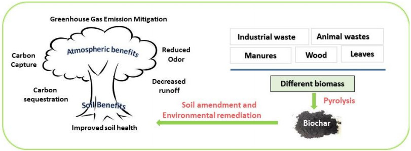
Biochar is a carbon-rich stable substance, defined as charred organic matter, produced during biomass thermochemical decomposition, and its application is currently considered as a mean of enhancing soil productivity, which is an important requirement for increasing crop yields whereas, simultaneously, it improves the quality of contaminated soil and water. However, depending on pedoclimatic conditions, its applicability exhibits negative aspects as well. It can also support biofuel production, therefore helping in reducing the demand for fossil fuels. Biochar is providing ecosystem services such as immobilization and transformation of contaminants and mitigation of climate change by sequestering carbon and reducing the release of greenhouse gases such as nitrous oxide and methane. It can further reduce waste as it could be produced from everything that contains biomass thereby assisting in waste management. Due to such wide-ranging applications, this review was conceptualized to emphasize the importance of biochar as an alternative to classic products used for energy, environmental and agricultural purposes. Based on the detailed information on the factors impacting biochar properties, the benefits and limitations of biochar, and the potential application guidelines for growers, this work aimed to help in partial achievement of multiple environmental goals and a practical recommendation to growers although its large-scale application is still controversial.
Citation: Shahram Torabian, Ruijun Qin, Christos Noulas, Yanyan Lu, Guojie Wang. Biochar: an organic amendment to crops and an environmental solution[J]. AIMS Agriculture and Food, 2021, 6(1): 401-415. doi: 10.3934/agrfood.2021024
Biochar is a carbon-rich stable substance, defined as charred organic matter, produced during biomass thermochemical decomposition, and its application is currently considered as a mean of enhancing soil productivity, which is an important requirement for increasing crop yields whereas, simultaneously, it improves the quality of contaminated soil and water. However, depending on pedoclimatic conditions, its applicability exhibits negative aspects as well. It can also support biofuel production, therefore helping in reducing the demand for fossil fuels. Biochar is providing ecosystem services such as immobilization and transformation of contaminants and mitigation of climate change by sequestering carbon and reducing the release of greenhouse gases such as nitrous oxide and methane. It can further reduce waste as it could be produced from everything that contains biomass thereby assisting in waste management. Due to such wide-ranging applications, this review was conceptualized to emphasize the importance of biochar as an alternative to classic products used for energy, environmental and agricultural purposes. Based on the detailed information on the factors impacting biochar properties, the benefits and limitations of biochar, and the potential application guidelines for growers, this work aimed to help in partial achievement of multiple environmental goals and a practical recommendation to growers although its large-scale application is still controversial.

| [1] |
El-Bassi L, Azzaz AA, Jellali S, et al. (2021) Application of olive mill waste-based biochars in agriculture: Impact on soil properties, enzymatic activities and tomato growth. Sci Total Environ 755: 142531. doi: 10.1016/j.scitotenv.2020.142531

|
| [2] |
Ahmad M, Rajapaksha AU, Lim JE, et al. (2014) Biochar as a sorbent for contaminant management in soil and water: A review. Chemosphere 99: 19–33. doi: 10.1016/j.chemosphere.2013.10.071
|
| [3] | Sohi S, Lopez-Capel E, Krull E, et al. (2009) Biochar, climate change and soil: A review to guide future research. CSIRO Land Water Sci Rep 5: 17–31. |
| [4] | Lehmann J, Joseph S (2009) Biochar for environmental management. Earthscan, Sterling, VA. |
| [5] |
Blanco-Canqui H (2017) Biochar and soil physical properties. Soil Sci Soc Am J 81: 687–711. doi: 10.2136/sssaj2017.01.0017
|
| [6] |
Agegnehu G, Bass AM, Nelson PN, et al. (2016) Benefits of biochar, compost and biochar–compost for soil quality, maize yield and greenhouse gas emissions in a tropical agricultural soil. Sci Total Environ 543: 295–306. doi: 10.1016/j.scitotenv.2015.11.054
|
| [7] | Gerlach H, Schmidt HP (2012) Biochar in poultry farming. Ithaka J 1: 262–264. |
| [8] |
Arif M, Ilyas M, Riaz M, et al. (2017) Biochar improves phosphorus use efficiency of organic-inorganic fertilizers, maize-wheat productivity and soil quality in a low fertility alkaline soil. Field Crops Res 214: 25–37. doi: 10.1016/j.fcr.2017.08.018
|
| [9] |
Meyer S, Glaser B, Quicker P (2011) Technical, economical, and climate-related aspects of biochar production technologies: a literature review. Environ Sci Technol 45: 9473–9483. doi: 10.1021/es201792c
|
| [10] |
Cha JS, Sun J, Park SH, et al. (2016) Production and utilization of biochar: A review. J Ind Eng Chem 40: 1–15. doi: 10.1016/j.jiec.2016.06.002
|
| [11] | Downie A, Crosky A, Munroe P (2009) Physical properties of biochar. In: Lehmann J, Joseph S (Eds), Biochar for environmental management: science and technology, Earthscan, London, 13–32. |
| [12] |
Ronsse F, van Hecke S, Dickinson D, et al. (2013) Production and characterization of slow pyrolysis biochar: Influence of feedstock type and pyrolysis conditions. GCB Bioenergy 5: 104–115. doi: 10.1111/gcbb.12018
|
| [13] |
Kloss S, Zehetner F, Dellantonio A, et al. (2012) Characterization of slow pyrolysis biochars: Effects of feedstocks and pyrolysis temperature on biochar properties. J Environ Qual 41: 990–1000. doi: 10.2134/jeq2011.0070
|
| [14] |
Laird D, Brown R, Amonette J, et al. (2009) Review of the pyrolysis platform for coproducing bio-oil and biochar. Biofuels Bioprod Biorefin 3: 547–562. doi: 10.1002/bbb.169
|
| [15] |
Sohi S, Krull E, Lopez-Capel E, et al. (2010) A review of biochar and its use and function in soil. Adv Agron 105: 47–82. doi: 10.1016/S0065-2113(10)05002-9
|
| [16] | Verheijen F, Jeffery S, Bastos AC, et al. (2010) Biochar application to soils. A critical scientific review of effects on soil properties, processes, and functions. EUR 24099: 162. |
| [17] |
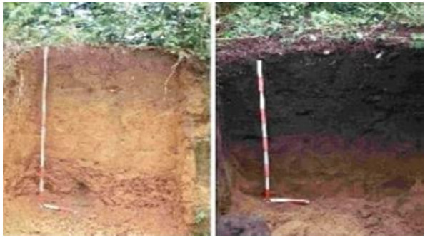
Lehmann J, da Silva JP, Steiner C, et al. (2003) Nutrient availability and leaching in an archaeological Anthrosol and a Ferralsol of the Central Amazon basin: Fertilizer, manure and charcoal amendments. Plant Soil 249: 343–357. doi: 10.1023/A:1022833116184
|
| [18] | Lehmann J (2009) Terra preta Nova – where to from here? In: Woods WI (Eds), Terra preta Nova: A Tribute to Wim Sombroek, Springer, Berlin, 473–486. |
| [19] |
Lu L, Yu W, Wang Y, et al. (2020) Application of biochar-based materials in environmental remediation: from multi-level structures to specific devices. Biochar 2: 1–31. doi: 10.1007/s42773-020-00041-7
|
| [20] |
Glaser B, Haumaier L, Guggenberger G, et al. (2001) The Terra Preta phenomenon: A model for sustainable agriculture in the humid tropics. Naturwissenschaften 88: 37–41. doi: 10.1007/s001140000193
|
| [21] | Glaser B, Guggenberger G, Zech W (2004) Identifying the Pre-Columbian anthropogenic input on present soil properties of Amazonian Dark Earth (Terra Preta). In: Glaser B, Woods W (Eds.), Amazonian Dark Earths: Explorations in Space and Time, Springer, Heidelberg, 215. |
| [22] |
Jeffery S, Verheijen FGA, van der Velde M, et al. (2011) A quantitative review of the effects of biochar application to soils on crop productivity using meta analysis. Agr Ecosyst Environ 144: 175–187. doi: 10.1016/j.agee.2011.08.015
|
| [23] |
Lee EH, Park RS, Kim H, et al. (2016) Hydrodeoxygenation of guaiacol over Pt loaded zeolitic materials. J Ind Eng Chem 37: 18–21. doi: 10.1016/j.jiec.2016.03.019
|
| [24] |
Han TU, Kim YM, Watanabe C, et al. (2015) Analytical pyrolysis properties of waste medium-density fiberboard and particle board. J Ind Eng Chem 32: 345–352. doi: 10.1016/j.jiec.2015.09.008
|
| [25] |
Heidari A, Stahl R, Younesi H, et al. (2014) Effect of process conditions on product yield and composition of fast pyrolysis of Eucalyptus grandis in fluidized bed reactor. J Ind Eng Chem 20: 2594–2602. doi: 10.1016/j.jiec.2013.10.046
|
| [26] |
Shafaghat H, Rezaei PS, Daud WMAW (2016) Catalytic hydrodeoxygenation of simulated phenolic bio-oil to cycloalkanes and aromatic hydrocarbons over bifunctional metal/acid catalysts of Ni/HBeta, Fe/HBeta and NiFe/HBeta. J Ind Eng Chem 35: 268–276. doi: 10.1016/j.jiec.2016.01.001
|
| [27] |
Fahmy TYA, Fahmy Y, Mobarak F, et al. (2020) Biomass pyrolysis: past, present, and future. Environ Dev Sustain 22: 17–32. doi: 10.1007/s10668-018-0200-5
|
| [28] | Brown R (2012) Biochar production technology. In: Biochar for environmental management, 159–178. |
| [29] |
Zhang H, Voroney RP, Price GW (2017) Effects of temperature and activation on biochar chemical properties and their impact on ammonium, nitrate, and phosphate sorption. J Environ Qual 46: 889–896. doi: 10.2134/jeq2017.02.0043
|
| [30] |
Leng L, Huang H, Li H, et al. (2019) Biochar stability assessment methods: a review. Sci Total Environ 647: 210–222. doi: 10.1016/j.scitotenv.2018.07.402
|
| [31] |
Bruun EW, Hauggaard-Nielsen H, Ibrahim N (2011) Influence of fast pyrolysis temperature on biochar labile fraction and short-term carbon loss in a loamy soil. Biomass Bioenerg 35: 1182–1189. doi: 10.1016/j.biombioe.2010.12.008
|
| [32] |
Wang D, Jiang P, Zhang H, et al. (2020) Biochar production and applications in agro and forestry systems: A review. Sci Total Environ 10: 137775. doi: 10.1016/j.scitotenv.2020.137775
|
| [33] |
Huber GW, Iborra S, Corman A (2006) Synthesis of transportation fuels from biomass; chemistry, catalysts, and engineering. Chem Rev 106: 4044–4098. doi: 10.1021/cr068360d
|
| [34] |
Zhang J, Liu J, Liu R (2015) Effects of pyrolysis temperature and heating time on biochar obtained from the pyrolysis of straw and lignosulfonate. Bioresour Technol 176: 288–291. doi: 10.1016/j.biortech.2014.11.011
|
| [35] |
Lu GQ, Low JCF, Liu CY, et al. (1995) Surface area development of sewage sludge during pyrolysis. Fuel 74: 344–348. doi: 10.1016/0016-2361(95)93465-P
|
| [36] |
Mohan D, Sarswat A, Ok YS, et al. (2014) Organic and inorganic contaminants removal from water with biochar, a renewable, low cost and sustainable adsorbent–a critical review. Bioresour Technol 160: 191–202. doi: 10.1016/j.biortech.2014.01.120
|
| [37] |
Lee Y, Park J, Ryu C, et al. (2013) Comparison of biochar properties from biomass residues produced by slow pyrolysis at 500 C. Bioresour Technol 148: 196–201. doi: 10.1016/j.biortech.2013.08.135
|
| [38] |
Evans MR, Jackson BE, Popp M, et al. (2017) Chemical properties of biochar materials manufactured from agricultural products common to the southeast United States. Horttechnology 27: 16–23. doi: 10.21273/HORTTECH03481-16
|
| [39] | Parmar A, Nema PK, Agarwal T (2014) Biochar production from agrofood industry residues: a sustainable approach for soil and environmental management. Curr Sci 107: 1673–1682. |
| [40] | Chan KY, Xu Z (2009) Biochar: nutrient properties and their enhancement. In: Lehmann J, Joseph S, Biochar for Environmental Management: Science and Technology, London: Earthscan, 67–84. |
| [41] |
Gao Y, Shao G, Lu J, et al. (2020) Effects of biochar application on crop water use efficiency depend on experimental conditions: A meta-analysis. Field Crops Res 249: 107763. doi: 10.1016/j.fcr.2020.107763
|
| [42] |
Xuan L, Yang Z, Zifu L, et al. (2014) Characterization of corncob derived biochar and pyrolysis kinetics in comparison with corn stalk and sawdust. Bioresour Technol 170: 76–82. doi: 10.1016/j.biortech.2014.07.077
|
| [43] |
Kan T, Strezov V, Evans TJ (2016) Lignocellulosic biomass pyrolysis: A review of product properties and effects of pyrolysis parameters. Renew Sustain Energy Rev 57: 1126–1140. doi: 10.1016/j.rser.2015.12.185
|
| [44] |
Peng X, Ye L, Wang C, et al. (2011) Temperature and duration dependent rice straw-derived biochar: characteristics and its effects on soil properties of an Ultisol in Southern China. Soil Tillage Res 112: 159–166. doi: 10.1016/j.still.2011.01.002
|
| [45] |
Si L, Xie Y, Ma Q, et al. (2018) The short-term effects of rice straw biochar, nitrogen and phosphorus fertilizer on rice yield and soil properties in a cold waterlogged paddy field. Sustainability 10: 537. doi: 10.3390/su10020537
|
| [46] |
Liu D, Feng Z, Zhu H, et al. (2020) Effects of Corn Straw Biochar Application on Soybean Growth and Alkaline Soil Properties. BioResources 15: 1463–1481. doi: 10.15376/biores.15.1.1463-1481
|
| [47] |
Taghizadeh-Toosi A, Clough TJ, Sherlock RR, et al. (2012) Biochar adsorbed ammonia is bioavailable. Plant Soil 350: 57–69. doi: 10.1007/s11104-011-0870-3
|
| [48] |
Ding Y, Liu Y, Liu S, et al. (2017) potential benefits of biochar in agricultural soils: A Review. Pedosphere 27: 645–661. doi: 10.1016/S1002-0160(17)60375-8
|
| [49] |
Pandit NR, Mulder J, Hale SE, et al. (2018) Biochar improves maize growth by alleviation of nutrient stress in a moderately acidic low-input Nepalese soil. Sci Total Environ 625: 1380–1389. doi: 10.1016/j.scitotenv.2018.01.022
|
| [50] |
Xu RK, Zhao AZ, Yuan JH, et al. (2012) pH buffering capacity of acid soils from tropical and subtropical regions of China as influenced by incorporation of crop straw biochars. J Soils Sediments 12: 494–502. doi: 10.1007/s11368-012-0483-3
|
| [51] |
Hussain R, Ravi K, Garg A (2020) Influence of biochar on the soil water retention characteristics (SWRC): potential application in geotechnical engineering structures. Soil Tillage Res 204: 104713. doi: 10.1016/j.still.2020.104713
|
| [52] | Kamran M, Malik Z, Parveen A, et al. (2020) Ameliorative effects of biochar on rapeseed (Brassica napus L.) growth and heavy metal immobilization in soil irrigated with untreated wastewater. J Plant Growth Regul 39: 266–281. |
| [53] |
Park JH, Choppala GK, Bolan N, et al. (2011) Biochar reduces the bioavailability and phytotoxicity of heavy metals. Plant Soil 348: 439–451. doi: 10.1007/s11104-011-0948-y
|
| [54] |
Abideen Z, Koyro HW, Huchzermeyer B, et al. (2020) Ameliorating effects of biochar on photosynthetic efficiency and antioxidant defence of Phragmites karka under drought stress. Plant Biol 22: 259–266. doi: 10.1111/plb.13054
|
| [55] |
Farhangi-Abriz S, Torabian S (2017) Antioxidant enzyme and osmotic adjustment changes in bean seedlings as affected by biochar under salt stress. Ecotoxicol Environ Saf 137: 64–70. doi: 10.1016/j.ecoenv.2016.11.029
|
| [56] |
Farhangi-Abriz S, Torabian S (2018) Effect of biochar on growth and ion contents of bean plant under saline condition. Environ Sci Pollut Res 25: 11556–11564. doi: 10.1007/s11356-018-1446-z
|
| [57] |
Elad Y, Rav David D, Meller Harel Y, et al. (2010) Induction of systemic resistance in plants by biochar, a soilapplied carbon sequestering agent. Phytopathology 100: 913–921. doi: 10.1094/PHYTO-100-9-0913
|
| [58] |
Elmer WH, Pignatello JJ (2011) Effect of biochar amendments on mycorrhizal associations and Fusarium crown and root rot of asparagus in replant soils. Plant Dis 95: 960–966. doi: 10.1094/PDIS-10-10-0741
|
| [59] | Nerome M, Toyota K, Islam TM, et al. (2005) Suppression of bacterial wilt of tomato by incorporation of municipal biowaste charcoal into soil. Soil Microorg (Japan) 59: 9–14. |
| [60] |
Song D, Chen L, Zhang S, et al. (2020) Combined biochar and nitrogen fertilizer change soil enzyme and microbial activities in a 2-year field trial. Eur J Soil Biol 99: 103212. doi: 10.1016/j.ejsobi.2020.103212
|
| [61] |
Lehmann J, Gaunt J, Rondon M (2006) Biochar sequestration in terrestrial ecosystems - a review. Mitig Adapt Strat GL 11: 403–427. doi: 10.1007/s11027-005-9006-5
|
| [62] |
Omondi MO, Xia X, Nahayo A, et al. (2016) Quantification of biochar effects on soil hydrological properties using meta-analysis of literature data. Geoderma 274: 28–34. doi: 10.1016/j.geoderma.2016.03.029
|
| [63] |
Jeffery S, Abalos D, Prodana M, et al. (2017) Biochar boosts tropical but not temperate crop yields. Environ Res Lett 12: 053001. doi: 10.1088/1748-9326/aa67bd
|
| [64] |
Ventura M, Alberti G, Panzacchi P, et al. (2019) Biochar mineralization and priming effect in a poplar short rotation coppice from a 3-year field experiment. Biol Fertil Soils 55: 67–78. doi: 10.1007/s00374-018-1329-y
|
| [65] |
Zimmerman AR, Ouyang L (2019) Priming of pyrogenic C (biochar) mineralization by dissolved organic matter and vice versa. Soil Biol Biochem 130: 105–112. doi: 10.1016/j.soilbio.2018.12.011
|
| [66] |
Cornelissen G, Nurida NL, Hale SE, et al. (2018) Fading positive effect of biochar on crop yield and soil acidity during five growth seasons in an Indonesian Ultisol. Sci Total Environ 634: 561–568. doi: 10.1016/j.scitotenv.2018.03.380
|
| [67] |
Van Zwieten L, Kimber S, Morris S, et al. (2010) Effects of biochar from slow pyrolysis of papermill waste on agronomic performance and soil fertility. Plant Soil 327: 235–246. doi: 10.1007/s11104-009-0050-x
|
| [68] | Glaser B, Lehr VI (2019) Biochar effects on phosphorus availability in agricultural soils: A meta-analysis. Sci Rep 9. |
| [69] |
Tammeorg P, Simojoki A, Mäkelä P, et al. (2014) Biochar application to a fertile sandy clay loam in boreal conditions: effects on soil properties and yield formation of wheat, turnip rape and faba bean. Plant Soil 374: 89–107. doi: 10.1007/s11104-013-1851-5
|
| [70] |
Liang F, Li GT, Lin QM, et al. (2014) Crop yield and soil properties in the first 3 years after biochar application to a calcareous soil. J Integr Agric 13: 525–532. doi: 10.1016/S2095-3119(13)60708-X
|
| [71] | Huang M, Long FAN, Jiang LG, et al. 2019. Continuous applications of biochar to rice: Effects on grain yield and yield attributes. J Integr Agric 18: 563–570. |
| [72] | Asai H, Samson BK, Stephan HM, et al. (2009) Biochar amendment techniques for upland rice production in northern laos: 1. soil physical properties, leaf SPAD and grain yield. Field Crop Res 111: 81–84. |
| [73] |
Lehmann J, Rillig MC, Thies J, et al. (2011) Biochar effects on soil biota–a review. Soil Biol Biochem 43: 1812–1836. doi: 10.1016/j.soilbio.2011.04.022
|
| [74] |
Noyce GL, Basiliko N, Fulthorpe R, et al. (2015) Soil microbial responses over 2 years following biochar addition to a north temperate forest. Biol Fertil Soils 51: 649–659. doi: 10.1007/s00374-015-1010-7
|
| [75] |
Wang N, Chang ZZ, Xue XM, et al. (2017) Biochar decreases nitrogen oxide and enhances methane emissions via altering microbial community composition of anaerobic paddy soil. Sci Total Environ 581: 689–696. doi: 10.1016/j.scitotenv.2016.12.181
|
| [76] |
Sarkhot DV, Berhe AA, Ghezzehei TA (2012) Impact of biochar enriched with dairy manure effluent on carbon and nitrogen dynamics. J Environ Qual 41: 1107–1114. doi: 10.2134/jeq2011.0123
|
| [77] |
Palansooriya KN, Wong JTF, Hashimoto Y, et al. (2019) Response of microbial communities to biochar-amended soils: a critical review. Biochar 1: 3–22. doi: 10.1007/s42773-019-00009-2
|
| [78] | Rasa K, Heikkinen J, Markus H, et al. (2018) How and why does willow biochar increase a clay soil water retention capacity? Biomass Bioenergy 119: 346–353. |
| [79] |
Zhang Y, Ding J, Wang H, et al. (2020) Biochar addition alleviate the negative effects of drought and salinity stress on soybean productivity and water use efficiency. BMC Plant Biol 20: 288. doi: 10.1186/s12870-020-02493-2
|
| [80] |
Zhang A, Liu Y, Pan G, et al. (2012) Effect of biochar amendment on maize yield and greenhouse gas emissions from a soil organic carbon poor calcareous loamy soil from Central China Plain. Plant Soil 351: 263–275. doi: 10.1007/s11104-011-0957-x
|
| [81] |
Guo M (2020) The 3R principles for applying biochar to improve soil health. Soil Syst 4: 9. doi: 10.3390/soilsystems4010009
|
| [82] | Lehmann J, Kern DC, Glaser B, et al. (2003) Amazonian Dark Earths: Origin, Properties, Management, Kluwer Academic Publishers, The Netherlands. |
| [83] |
Steiner C, Das KC, Garcia M, et al. (2008) Charcoal and smoke extract stimulate the soil microbial community in a highly weathered xanthic Ferralsol. Pedobiologia 51: 359–366. doi: 10.1016/j.pedobi.2007.08.002
|
| [84] |
Kolb SE, Fermanich KJ, Dornbush ME (2009) Effect of charcoal quantity on microbial biomass and activity in temperate soils. Soil Sci Soc Am J 73: 1173–1181. doi: 10.2136/sssaj2008.0232
|
| [85] |
Li S, Zhang Y, Yan W, et al. (2018) Effect of biochar application method on nitrogen leaching and hydraulic conductivity in a silty clay soil. Soil Tillage Res 183: 100–108. doi: 10.1016/j.still.2018.06.006
|
| [86] |
Cetin E, Moghtaderi B, Gupta R, et al. (2004) Influence of pyrolysis conditions on the structure and gasification reactivity of biomass chars. Fuel 83: 2139–2150. doi: 10.1016/j.fuel.2004.05.008
|
| [87] | Liu Z, Dugan B, Masiello CA, et al. (2017) Biochar particle size, shape, and porosity act together to influence soil water properties. Plos One 12: e0179079. |
| [88] |
Głąb T, Palmowska J, Zaleski T, et al. (2016) Effect of biochar application on soil hydrological properties and physical quality of sandy soil. Geoderma 281: 11–20. doi: 10.1016/j.geoderma.2016.06.028
|
| [89] |
Githinji L (2014) Effect of biochar application rate on soil physical and hydraulic properties of a sandy loam. Arch Agron Soil Sci 60: 457–470. doi: 10.1080/03650340.2013.821698
|
| [90] | Robb S, Joseph S (2019) A Report on the value of biochar and wood vinegar: Practical experience of users in Australia and New Zealand; Australia New Zealand Biochar Initiative, Inc.: Tyagarah, Australia, 2019; Available from: https://www.anzbi.org/wp-content/uploads/2019/06/ANZBI-2019-_-A-Report-on-the-Value-of-Biochar-and-Wood-Vinegar-v-1.1.pdf (accessed on 01 October 2020). |
| [91] | Maroušková A, Braun P (2014) Holistic approach to improve the energy utilization of Jatropha curcas L. Rev Téc Ing Univ Zulia 37: 144–150. |
Figures(2) / Tables(1)

Shahram Torabian, Ruijun Qin, Christos Noulas, Yanyan Lu, Guojie Wang. Biochar: an organic amendment to crops and an environmental solution[J]. AIMS Agriculture and Food, 2021, 6(1): 401-415. doi: 10.3934/agrfood.2021024


 DownLoad: