Cecum microbiota in rats fed soy, milk, meat, fish, and egg proteins with prebiotic oligosaccharides

Souliphone Sivixay; Gaowa Bai; Takeshi Tsuruta; Naoki Nishino; Souliphone Sivixay; Gaowa Bai; Takeshi Tsuruta; Naoki Nishino

doi:10.3934/microbiol.2021001

AIMS Microbiology

2021, Volume 7, Issue 1: 1-12. doi: 10.3934/microbiol.2021001

Previous Article Next Article

Research article

Cecum microbiota in rats fed soy, milk, meat, fish, and egg proteins with prebiotic oligosaccharides

1.
Department of Animal Science, Graduate School of Life and Environmental Science, Okayama University, Okayama, Japan
2.
Department of Health Science and Social Welfare, Takahashi, Japan

Received: 03 November 2020 Accepted: 12 January 2021 Published: 14 January 2021

Diet is considered the most influential factor in modulating the gut microbiota but how dietary protein sources differ in their modulatory effects is not well understood. In this study, soy, meat (mixture of beef and pork), and fish proteins (experiment 1) and soy, milk (casein), and egg proteins (experiment 2) were fed to rats with cellulose (CEL) and raffinose (RAF); the microbiota composition and short-chain fatty acid concentration in the cecum were determined. Egg protein feeding decreased the concentration of acetic acid and the richness and diversity of the cecum microbiota. RAF feeding increased the concentrations of acetic and propionic acids and decreased the richness and diversity of the cecum microbiota. When fed with CEL, the abundance of Ruminococcaceae and Christensenellaceae, Akkermansiaceae and Tannerellaceae, and Erysipelotrichaceae enhanced with soy protein, meat and fish proteins, and egg protein, respectively. The effects of dietary proteins diminished with RAF feeding and the abundance of Bifidobacteriaceae, Erysipelotrichaceae, and Lachnospiraceae increased and that of Ruminococcaceae and Christensenellaceae decreased regardless of the protein source. These results indicate that, although the effect of prebiotics is more robust and distinctive, dietary protein sources may influence the composition and metabolic activities of the gut microbiota. The stimulatory effects of soy, meat, and egg proteins on Christensenellaceae, Akkermansiaceae, and Erysipelotrichaceae deserve further examination to better elucidate the dietary manipulation of the gut microbiota.

Keywords:

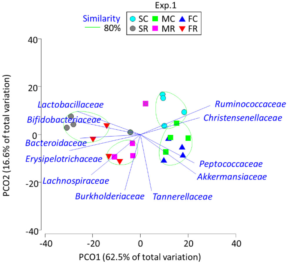
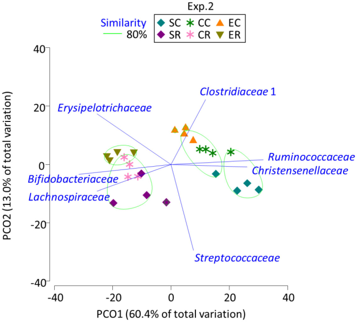
Citation: Souliphone Sivixay, Gaowa Bai, Takeshi Tsuruta, Naoki Nishino. Cecum microbiota in rats fed soy, milk, meat, fish, and egg proteins with prebiotic oligosaccharides[J]. AIMS Microbiology, 2021, 7(1): 1-12. doi: 10.3934/microbiol.2021001

Related Papers:

[1]	M. Botros, E. A. A. Ziada, I. L. EL-Kalla . Semi-analytic solutions of nonlinear multidimensional fractional differential equations. Mathematical Biosciences and Engineering, 2022, 19(12): 13306-13320. doi: 10.3934/mbe.2022623
[2]	Yan Xie, Zhijun Liu, Ke Qi, Dongchen Shangguan, Qinglong Wang . A stochastic mussel-algae model under regime switching. Mathematical Biosciences and Engineering, 2022, 19(5): 4794-4811. doi: 10.3934/mbe.2022224
[3]	Debao Yan . Existence results of fractional differential equations with nonlocal double-integral boundary conditions. Mathematical Biosciences and Engineering, 2023, 20(3): 4437-4454. doi: 10.3934/mbe.2023206
[4]	Ilse Domínguez-Alemán, Itzel Domínguez-Alemán, Juan Carlos Hernández-Gómez, Francisco J. Ariza-Hernández . A predator-prey fractional model with disease in the prey species. Mathematical Biosciences and Engineering, 2024, 21(3): 3713-3741. doi: 10.3934/mbe.2024164
[5]	Zahra Eidinejad, Reza Saadati . Hyers-Ulam-Rassias-Kummer stability of the fractional integro-differential equations. Mathematical Biosciences and Engineering, 2022, 19(7): 6536-6550. doi: 10.3934/mbe.2022308
[6]	Reymundo Itzá Balam, Francisco Hernandez-Lopez, Joel Trejo-Sánchez, Miguel Uh Zapata . An immersed boundary neural network for solving elliptic equations with singular forces on arbitrary domains. Mathematical Biosciences and Engineering, 2021, 18(1): 22-56. doi: 10.3934/mbe.2021002
[7]	Qiong Wu, Zhimin Yao, Zhouping Yin, Hai Zhang . Fin-TS and Fix-TS on fractional quaternion delayed neural networks with uncertainty via establishing a new Caputo derivative inequality approach. Mathematical Biosciences and Engineering, 2022, 19(9): 9220-9243. doi: 10.3934/mbe.2022428
[8]	Sebastian Builes, Jhoana P. Romero-Leiton, Leon A. Valencia . Deterministic, stochastic and fractional mathematical approaches applied to AMR. Mathematical Biosciences and Engineering, 2025, 22(2): 389-414. doi: 10.3934/mbe.2025015
[9]	Lin Zhang, Yongbin Ge, Xiaojia Yang . High-accuracy positivity-preserving numerical method for Keller-Segel model. Mathematical Biosciences and Engineering, 2023, 20(5): 8601-8631. doi: 10.3934/mbe.2023378
[10]	P. Auger, N. H. Du, N. T. Hieu . Evolution of Lotka-Volterra predator-prey systems under telegraph noise. Mathematical Biosciences and Engineering, 2009, 6(4): 683-700. doi: 10.3934/mbe.2009.6.683

Abstract

1. Introduction

In this paper we study the following time-fractional telegraph equation (TFTE) ^[1,2,3]

$\begin{eqnarray} \left\{ \begin{array}{ll} D_{C, t}^{\gamma}u(x, t)+aD_{C, t}^{\gamma-1}u(x, t)+bu(x, t) = cu_{xx}(x, t)+f(x, t), & (x, t)\in (0, 1)\times (0, T], \\ u(x, 0) = \phi_{1}(x), \ \ u_{t}(x, 0) = \phi_{2}(x), & x\in [0, 1], \\ u(0, t) = \psi_{1}(t), \ \ u(1, t) = \psi_{2}(t), & t\in [0, T], \end{array} \right. \end{eqnarray}$

(1.1)

where $1 < \gamma < 2$ , $a, b, c$ and $T$ are given positive constants, $f(x, t), \phi_{1}(x), \phi_{2}(x), \psi_{1}(t)$ and $\psi_{2}(t)$ are given functions and satisfy the compatibility conditions, $D_{C, t}^{\gamma}u(x, t)$ and $D_{C, t}^{\gamma-1}u(x, t)$ are the Caputo fractional derivatives of order $\gamma$ and $\gamma-1$ respectively. The Caputo fractional derivative $D_{C, t}^{\gamma}u(x, t)$ is defined by ^[4,Definition 2.2]

$\begin{eqnarray*} D^{\gamma}_{C, t}u(x, t) = \frac{1}{\Gamma(2-\gamma)}\int_{0}^{t}\left(t-s\right)^{1-\gamma}u_{ss}(x, s){\rm d}s. \end{eqnarray*}$

The Caputo operators $D_{C, t}^{\gamma}$ and $D_{C, t}^{\gamma-1}$ have the following relationship

$\begin{eqnarray*} D^{\gamma}_{C, t}u(x, t) = \frac{1}{\Gamma\left(1-(\gamma-1)\right)}\int_{0}^{t}\left(t-s\right)^{-(\gamma-1)}\frac{\partial}{\partial s}u_{s}(x, s){\rm d}s = D^{\gamma-1}_{C, t}u_{t}(x, t). \end{eqnarray*}$

Based on the above relationship, the TFTE (1.1) can be transformed into the following equivalent integral-differential equation as shown in ^[4,Lemma 6.2]

$\begin{eqnarray} \left\{ \begin{array}{ll} u_{t}(x, t)+au(x, t) = a\phi_{1}(x)+\phi_{2}(x)\\ +\frac{1}{\Gamma(\gamma-1)}\int_{0}^{t}\left(t-s\right)^{\gamma-2}\left[cu_{xx}(x, s)-bu(x, s)+f(x, s)\right]{\rm d}s, & (x, t)\in (0, 1)\times (0, T], \\ u(x, 0) = \phi_{1}(x), & x\in [0, 1], \\ u(0, t) = \psi_{1}(t), \ \ u(1, t) = \psi_{2}(t), & t\in [0, T], \end{array} \right. \end{eqnarray}$

(1.2)

which simplifies the original problem to a certain extent. For the subsequent numerical discretization and error analysis, we assume

$\begin{eqnarray} \left|\frac{\partial^{l}f(x, t)}{\partial t^{l}}\right|\leq C\left(1+t^{\gamma-l}\right), \ \ \ \ \ \ \ \ \ \ \ \ l = 0, 1, 2. \end{eqnarray}$

(1.3)

The TFTE (1.1) is used to describe some phenomena such as propagation of electric signals ^[5], acoustic waves in porous media ^[6], transport of neutron in a nuclear reactor ^[7], and hyperbolic heat transfer ^[8].

There are a few numerical methods to solve the TFTE. Wang ^[9] developed a method in the reproducing kernel space by piecewise technique to solve the TFTE. Hosseini et al. ^[10] applied the radial basis functions and finite difference method to solve the TFTE. Kumar et al. ^[11] described a finite difference scheme for the generalized TFTE. Hashemi and Baleanu ^[12] utilized a combination of method of line and group preserving scheme to solve the TFTE. Wei et al. ^[13] discussed a fully discrete local discontinuous Galerkin finite element method for the TFTE. Sweilam ^[14] introduced the Sinc-Legendre collocation method for solving the TFTE. Mollahasani et al. ^[15] presented an operational method based on hybrid functions of Legendre polynomials and Block-Pulse-Functions for solving the TFTE. Hafez and Youssri ^[16] used a shifted Jacobi collocation scheme for a multidimensional TFTE. Bhrawy et al. ^[17] proposed an accurate and efficient spectral algorithm for the numerical solution of the two-sided space-time TFTE with three types of non-homogeneous boundary conditions. Youssri et al. ^[18,19] also developed numerical spectral Legendre approaches to solve the TFTEs. Bhrawy and Zaky ^[20] used a method based on the Jacobi tau approximation for solving multi-term time-space TFTE. In ^[2,3] B-spline collocation methods were applied to solve the TFTEs. In ^[21,22] wavelet methods were used to solve the TFTEs. But these papers only study the case that the solutions of the TFTEs are sufficiently smooth. Special treatment techniques, such as graded meshes ^{[23,24,25,26,27]} and mapped basis functions ^[28] reflecting the characteristics of the singularity of the exact solution, need to be used to solve the fractional differential equations.

The aim of the present study is twofold. The first aim is to construct an integral-difference discretization scheme on a graded mesh to approximate the integral-differential equation with a weakly singular kernel transformed from the TFTE, which is a second-order convergence discretization scheme. The second aim is to take the possible singularity of the exact solution into account in the convergence analysis, where the singularity of the exact solution is reflected as

$\begin{eqnarray} \left|\frac{\partial^{k}u(x, t)}{\partial x^{k}}\right|\leq C, \ \ \ \ \ \ \ \ \ \ \ \ \ \ \ \ \, \ \ \ \ \ \ k = 0, 1, \dots, 4, \end{eqnarray}$

(1.4)

$\begin{eqnarray} \left|\frac{\partial^{l+m}u(x, t)}{\partial t^{l}\partial x^{m}}\right|\leq C\left(1+t^{\gamma-l}\right), \ \ \ \ \ \ l = 0, 1, 2, 3, \ \ {\rm and}\ \ m = 0, 1, 2, \end{eqnarray}$

(1.5)

which can be referred in the literature ^{[25,26,27,29]} for details. We show that our discretization scheme on a graded mesh is second-order convergent for both the spatial discretization and the time discretization, although the exact solution of the TFTE may have singularity. Numerical experiments confirm the effectiveness of the theoretical results, and also verify that this scheme is more accurate than the methods given in ^[2,3].

Remark 1.1 If $b, c$ are variable coefficients and $a$ is a variable coefficient with respect to $x$ , the TFTE (1.1) can also be transformed into the same integral-differential equation as given in (1.2). If $a$ is a variable coefficient with respect to $t$ , we first approximate $a$ with a piecewise linear interpolation function about $t$ and then transform the approximate TFTE into an integral-differential equation as given in (1.2). If there is a nonlinear term in the TFTE, we first transform it into a linear equation by Newton iterative method and then transform it into an integral-differential equation as given in (1.2).

Notation. Throughout the paper, $C$ is used to indicate the positive constant independent of the mesh, and $C$ in different places can represent different values. In order to simplify the notation, the representation $g_{i}^{j} = g(x_{i}, t_{j})$ is introduced for any function $g$ at the mesh point $(x_{i}, t_{j})\in (0, 1)\times (0, T]$ .

2. Discretization scheme

We developed the discretization scheme on a graded mesh $\bar{\Omega}^{N, K}\equiv\left\{\left(x_{i}, t_{j}\right)\left|x_{i} = ih, h = 1/N, 0\leq i\leq \right.\right.$ $\left. N, 0\leq j\leq K \right\}$ with time mesh points

$\begin{eqnarray} t_{j} = T\left(\frac{j}{K}\right)^{\frac{2}{\gamma-1}} \end{eqnarray}$

(2.1)

and time sizes $\triangle t_{j} = t_{j}-t_{j-1}$ for $1\leq j\leq K$ , where the discretization parameters $N$ and $K$ are positive integers. The following integral-difference discretization scheme

$\begin{array}{l} \frac{U_{i}^{j}-U_{i}^{j-1}}{\triangle t_{j}}+a\frac{U_{i}^{j-1}+U_{i}^{j}}{2}\nonumber\\ = a\phi_{1, i}+\phi_{2, i} +\frac{1}{2\Gamma(\gamma-1)}\sum\limits_{k = 1}^{j-1}\int_{t_{k-1}}^{t_{k}}\left(t_{j-1}-s\right)^{\gamma-2}\left[\frac{t_{k}-s}{\triangle t_{k}}\left(c\delta^{2}_{x} U_{i}^{k-1}-bU_{i}^{k-1}+f_{i}^{k-1}\right) \right. \nonumber\\ \ \ \ \left. +\frac{s-t_{k-1}}{\triangle t_{k}}\left(c\delta^{2}_{x} U_{i}^{k}-bU_{i}^{k}+f_{i}^{k}\right)\right]{\rm d}s+\frac{1}{2\Gamma(\gamma-1)}\sum\limits_{k = 1}^{j}\int_{t_{k-1}}^{t_{k}}\left(t_{j}-s\right)^{\gamma-2}\nonumber\\ \ \ \ \cdot \left[\frac{t_{k}-s}{\triangle t_{k}}\left(c\delta^{2}_{x} U_{i}^{k-1}-bU_{i}^{k-1}+f_{i}^{k-1}\right) +\frac{s-t_{k-1}}{\triangle t_{k}}\left(c\delta^{2}_{x} U_{i}^{k}-bU_{i}^{k}+f_{i}^{k}\right)\right]{\rm d}s \end{array}$

for $1\leq i < N$ and $1\leq j\leq K$ is used to approximate the integral-differential equation in (1.2), where $U_{i}^{j}$ denotes the numerical solution at the mesh point $\left(x_{i}, t_{j}\right)$ and $\delta^{2}_{x} U_{i}^{j} = \frac{U_{i+1}^{j}-2U_{i}^{j}+U_{i-1}^{j}}{h^{2}}$ . Thus, our discretization scheme for problem (1.2) is

$\begin{eqnarray} \left\{ \begin{array}{ll} \frac{U_{i}^{j}-U_{i}^{j-1}}{\triangle t_{j}}+a\frac{U_{i}^{j-1}+U_{i}^{j}}{2} = a\phi_{1, i}+\phi_{2, i}\\ {+ \frac{1}{2}\sum\limits_{k = 1}^{j-1}\left[\xi_{j-1, k}\left(c\delta^{2}_{x} U_{i}^{k-1}-bU_{i}^{k-1}+f_{i}^{k-1}\right)+\eta_{j-1, k}\left(c\delta^{2}_{x} U_{i}^{k}-bU_{i}^{k}+f_{i}^{k}\right)\right]}\\ {+ \frac{1}{2}\sum\limits_{k = 1}^{j}\left[\xi_{j, k}\left(c\delta^{2}_{x} U_{i}^{k-1}-bU_{i}^{k-1}+f_{i}^{k-1}\right)+\eta_{j, k}\left(c\delta^{2}_{x} U_{i}^{k}-bU_{i}^{k}+f_{i}^{k}\right)\right]}, & 1\leq i < N, 1\leq j\leq K, \\ U_{i}^{0} = \phi_{1}(x_{i}), & 0\leq i\leq N, \\ U_{0}^{j} = \psi_{1}(t_{j}), \ \ U_{N}^{j} = \psi_{2}(t_{j}), & 1\leq j\leq K, \end{array} \right. \end{eqnarray}$

(2.2)

where

$\begin{eqnarray} \xi_{j, k} = \frac{1}{\triangle t_{k}\Gamma(\gamma-1)}\int_{t_{k-1}}^{t_{k}}\left(t_{j}-s\right)^{\gamma-2}\left(t_{k}-s\right){\rm d}s, \ \ \ \ \ \ \ \ \ \ \ \ k = 1, 2\dots, j, \end{eqnarray}$

(2.3)

$\begin{eqnarray} \eta_{j, k} = \frac{1}{\triangle t_{k}\Gamma(\gamma-1)}\int_{t_{k-1}}^{t_{k}}\left(t_{j}-s\right)^{\gamma-2}\left(s-t_{k-1}\right){\rm d}s, \ \ \ \ \ \ \ \ \ k = 1, 2\dots, j. \end{eqnarray}$

(2.4)

Let $z_{i}^{j} = U_{i}^{j}-u_{i}^{j}$ for $0\leq i\leq N$ and $0\leq j\leq K$ . Then, from (1.2) and (2.2) we know that the error mesh function $z$ satisfies

$\begin{eqnarray} \left\{ \begin{array}{ll} \frac{z_{i}^{j}-z_{i}^{j-1}}{\triangle t_{j}}+a\frac{z_{i}^{j-1}+z_{i}^{j}}{2}\\ { = \frac{1}{2}\sum\limits_{k = 1}^{j-1}\left[\xi_{j-1, k}\left(c\delta^{2}_{x} z_{i}^{k-1}-bz_{i}^{k-1}\right)+\eta_{j-1, k}\left(c\delta^{2}_{x} z_{i}^{k}-bz_{i}^{k}\right)\right]}\\ \ \ \ {+ \frac{1}{2}\sum\limits_{k = 1}^{j}\left[\xi_{j, k}\left(c\delta^{2}_{x} z_{i}^{k-1}-bz_{i}^{k-1}\right)+\eta_{j, k}\left(c\delta^{2}_{x} z_{i}^{k}-bz_{i}^{k}\right)\right]}+R_{i}^{j}, & 1\leq i < N, 1\leq j\leq K, \\ z_{i}^{0} = 0, & 0\leq i\leq N, \\ z_{0}^{j} = z_{N}^{j} = 0, & 1\leq j\leq K, \end{array} \right. \end{eqnarray}$

(2.5)

where

$\begin{eqnarray*} R_{i}^{j} & = & \frac{1}{2}\left(\frac{\partial u}{\partial t}(x_{i}, t_{j-1})+\frac{\partial u}{\partial t}(x_{i}, t_{j})\right)-\frac{u_{i}^{j}-u_{i}^{j-1}}{\triangle t_{j}}\nonumber\\ & & +\frac{1}{2\Gamma(\gamma-1)}\sum\limits_{k = 1}^{j-1}\int_{t_{k-1}}^{t_{k}}\left(t_{j-1}-s\right)^{\gamma-2}\left[\frac{t_{k}-s}{\triangle t_{k}}\left(c\delta^{2}_{x} u_{i}^{k-1}-bu_{i}^{k-1}+f_{i}^{k-1}\right)\right.\nonumber\\ & & \left. +\frac{s-t_{k-1}}{\triangle t_{k}}\left(c\delta^{2}_{x} u_{i}^{k}-bu_{i}^{k}+f_{i}^{k}\right)-\left(c\frac{\partial^{2} u(x_{i}, s)}{\partial x^{2}}-bu\left(x_{i}, s\right)+f\left(x_{i}, s\right)\right)\right]{\rm d}s\nonumber\\ & & +\frac{1}{2\Gamma(\gamma-1)}\sum\limits_{k = 1}^{j}\int_{t_{k-1}}^{t_{k}}\left(t_{j}-s\right)^{\gamma-2}\left[\frac{t_{k}-s}{\triangle t_{k}}\left(c\delta^{2}_{x} u_{i}^{k-1}-bu_{i}^{k-1}+f_{i}^{k-1}\right)\right.\nonumber\\ & & \left. +\frac{s-t_{k-1}}{\triangle t_{k}}\left(c\delta^{2}_{x} u_{i}^{k}-bu_{i}^{k}+f_{i}^{k}\right)-\left(c\frac{\partial^{2} u(x_{i}, s)}{\partial x^{2}}-bu\left(x_{i}, s\right)+f\left(x_{i}, s\right)\right)\right]{\rm d}s. \end{eqnarray*}$

Then, under the assumption (1.3) we can obtain

$\begin{eqnarray} \left|R_{i}^{j}\right| & \leq & C\int_{t_{j-1}}^{t_{j}}\left|\frac{\partial^{3}u}{\partial s^{3}}\left(x_{i}, s\right)\right|\left(s-t_{j-1}\right){\rm d}s +C\sum\limits_{k = 1}^{j-1}\int_{t_{k-1}}^{t_{k}}\left(t_{j-1}-s\right)^{\gamma-2}\left\{\frac{t_{k}-s}{\triangle t_{k}}\left(s-t_{k-1}\right)^{2}\right.\\ & & \left. \cdot\left|\int_{0}^{1} \left(c\frac{\partial^{4} u}{\partial x^{2}\partial t^{2}}-b\frac{\partial^{2} u}{\partial t^{2}} +\frac{\partial^{2} f}{\partial t^{2}}\right)\left(x_{i}, t_{k-1}+\left(s-t_{k-1}\right)y\right)y{\rm d}y\right|\right.\\ & & \left.+\frac{s-t_{k-1}}{\triangle t_{k}}\left(t_{k}-s\right)^{2}\left|\int_{0}^{1} \left(c\frac{\partial^{4} u}{\partial x^{2}\partial t^{2}}-b\frac{\partial^{2} u}{\partial t^{2}}+\frac{\partial^{2} f}{\partial t^{2}}\right) \left(x_{i}, s+\left(t_{k}-s\right)y\right)\left(1-y\right){\rm d}y\right|\right\}{\rm d}s\\ & & +C\sum\limits_{k = 1}^{j}\int_{t_{k-1}}^{t_{k}}\left(t_{j}-s\right)^{\gamma-2}\left\{\frac{t_{k}-s}{\triangle t_{k}}\left(s-t_{k-1}\right)^{2}\right.\\ & & \left. \cdot\left|\int_{0}^{1} \left(c\frac{\partial^{4} u}{\partial x^{2}\partial t^{2}}-b\frac{\partial^{2} u}{\partial t^{2}} +\frac{\partial^{2} f}{\partial t^{2}}\right)\left(x_{i}, t_{k-1}+\left(s-t_{k-1}\right)y\right)y{\rm d}y\right|\right.\\ & & \left.+\frac{s-t_{k-1}}{\triangle t_{k}}\left(t_{k}-s\right)^{2}\left|\int_{0}^{1} \left(c\frac{\partial^{4} u}{\partial x^{2}\partial t^{2}}-b\frac{\partial^{2} u}{\partial t^{2}}+\frac{\partial^{2} f}{\partial t^{2}}\right) \left(x_{i}, s+\left(t_{k}-s\right)y\right)\left(1-y\right){\rm d}y\right|\right\}{\rm d}s\\ & & +C\sum\limits_{k = 1}^{j-1}\int_{t_{k-1}}^{t_{k}}\left(t_{j-1}-s\right)^{\gamma-2}\left|\frac{t_{k}-s}{\triangle t_{k}}\left(\delta^{2}_{x} u_{i}^{k-1}-\frac{\partial^{2}u\left(x_{i}, t_{k-1}\right)}{\partial x^{2}}\right)\right.\\ & & \left. +\frac{s-t_{k-1}}{\triangle t_{k}}\left(\delta^{2}_{x} u_{i}^{k}-\frac{\partial^{2}u\left(x_{i}, t_{k}\right)}{\partial x^{2}}\right)\right|{\rm d}s\\ & & +C\sum\limits_{k = 1}^{j}\int_{t_{k-1}}^{t_{k}}\left(t_{j}-s\right)^{\gamma-2}\left|\frac{t_{k}-s}{\triangle t_{k}}\left(\delta^{2}_{x} u_{i}^{k-1}-\frac{\partial^{2}u\left(x_{i}, t_{k-1}\right)}{\partial x^{2}}\right)\right.\\ & & \left. +\frac{s-t_{k-1}}{\triangle t_{k}}\left(\delta^{2}_{x} u_{i}^{k}-\frac{\partial^{2}u\left(x_{i}, t_{k}\right)}{\partial x^{2}}\right)\right|{\rm d}s\\ &\leq & C\left(\int_{t_{j-1}}^{t_{j}}s^{\frac{\gamma-3}{2}}{\rm d}s\right)^{2}+ C\sum\limits_{k = 1}^{j-1}\triangle t_{k}\int_{t_{k-1}}^{t_{k}}\left(t_{j-1}-s\right)^{\gamma-2}\int_{t_{k-1}}^{t_{k}}t^{\gamma-2}{\rm d}t{\rm d}s\\ & & + C\sum\limits_{k = 1}^{j}\triangle t_{k}\int_{t_{k-1}}^{t_{k}}\left(t_{j}-s\right)^{\gamma-2}\int_{t_{k-1}}^{t_{k}}t^{\gamma-2}{\rm d}t{\rm d}s+Ch^{2}\\ & \leq & C\left(N^{-2}+K^{-2}\right), \end{eqnarray}$

(2.6)

where we have used the linear interpolation remainder formula

$\begin{eqnarray*} \frac{t_{k}-t}{\triangle t_{k}}g_{k-1}+\frac{t-t_{k-1}}{\triangle t_{k}}g_{k}-g(t) & = & \frac{1}{\triangle t_{k}}\left\{\left(t_{k}-t\right)\left(t-t_{k-1}\right)^{2}\int_{0}^{1}g''\left[t_{k-1}+\left(t-t_{k-1}\right)s\right]s{\rm d}s\right.\nonumber\\ & & \left.+\left(t-t_{k-1}\right)\left(t_{k}-t\right)^{2}\int_{0}^{1}g''\left[t+\left(t_{k}-t\right)s\right]\left(1-s\right){\rm d}s\right\}, \end{eqnarray*}$

the regularities (1.4) and (1.5), the assumption (1.3), the graded mesh (2.1), the inequality (see ^[30])

$\begin{eqnarray*} \int_{t_{j-1}}^{t_{j}}s^{\alpha}\left(s-t_{j-1}\right){\rm d}s\leq \frac{1}{2}\left\{\int_{t_{j-1}}^{t_{j}}s^{\alpha/2}{\rm d}s\right\}^{2} \end{eqnarray*}$

for $\alpha < 0$ , and the following estimates

$\begin{array}{l} \int_{t_{j-1}}^{t_{j}}s^{\frac{\gamma-3}{2}}{\rm d}s = \frac{2}{\gamma-1}\left(t_{j}^{\frac{\gamma-1}{2}}-t_{j-1}^{\frac{\gamma-1}{2}}\right)\leq CK^{-1}, \\ \triangle t_{1}\int_{0}^{t_{1}}\left(t_{j}-s\right)^{\gamma-2}\int_{0}^{t_{1}}t^{\gamma-2}{\rm d}t{\rm d}s\leq C\left(\triangle t_{1}\right)^{\gamma}\int_{0}^{t_{1}}\left(t_{j}-s\right)^{\gamma-2}{\rm d}s\leq C\left(\frac{1}{K}\right)^{\frac{2\gamma}{\gamma-1}}\leq CK^{-2\gamma}, \\ \sum\limits_{k = 2}^{j}\triangle t_{k}\int_{t_{k-1}}^{t_{k}}\left(t_{j}-s\right)^{\gamma-2}\int_{t_{k-1}}^{t_{k}}t^{\gamma-2}{\rm d}t{\rm d}s\leq C\sum\limits_{k = 2}^{j}\left(\triangle t_{k}\right)^{3}\left(t_{j}-t_{k-1}\right)^{\gamma-2}t_{k-1}^{\gamma-2}\nonumber\\ = C \sum\limits_{k = 2}^{j}\left[\left(\frac{k}{K}\right)^\frac{2}{\gamma-1}- \left(\frac{k-1}{K}\right)^\frac{2}{\gamma-1}\right]^{3}\left[t_{j}-\left(\frac{k-1}{K}\right)^{\frac{2}{\gamma-1}}\right]^{\gamma-2} \left(\frac{k-1}{K}\right)^{\frac{2\left(\gamma-2\right)}{\gamma-1}}\nonumber\\ \leq CK^{-3} \sum\limits_{k = 1}^{j}\left(\frac{k}{K}\right)^{\frac{6}{\gamma-1}-3}\left(t_{j}-\frac{k-1}{K}\right)^{\gamma-2}\left(\frac{k-1}{K}\right)^{\frac{2\left(\gamma-2\right)}{\gamma-1}}\nonumber\\ \leq CK^{-2} \sum\limits_{k = 1}^{j-1}\left(t_{j}-\frac{k}{K}\right)^{\gamma-2}\left(\frac{k}{K}\right)^{\frac{5-\gamma}{\gamma-1}}\frac{1}{K}\nonumber\\ \leq CK^{-2}\int_{0}^{t_{j}}\left(t_{j}-s\right)^{\gamma-2}s^{\frac{5-\gamma}{\gamma-1}}{\rm d}s \nonumber\\ = CK^{-2}t_{j}^{\gamma-1+\frac{5-\gamma}{\gamma-1}}B\left(\frac{4}{\gamma-1}, \gamma-1\right)\nonumber\\ \leq CK^{-2}. \end{array}$

The following lemma gives a useful result for our convergence analysis, which is given in ^[31].

Lemma 2.1 Assume that $\left\{\omega_{k}\right\}_{k = 0}^{\infty}$ be a sequence of non-negative real numbers satisfying

$\begin{eqnarray*} \omega_{k}\geq 0, \ \ \ \omega_{k+1}\leq \omega_{k}, \ \ \ \omega_{k+1}-2\omega_{k}+\omega_{k-1}\geq 0. \end{eqnarray*}$

Then for any integer $K > 0$ and vector $\left(V_{1}, V_{2}, \dots, V_{K}\right)^{T}\in \mathbb{R}^{K}$ , the following inequality

$\begin{eqnarray*} \sum\limits_{k = 1}^{K}\left(\sum\limits_{p = 1}^{k}\omega_{k-p}V_{p}\right)V_{k}\geq 0 \end{eqnarray*}$

holds true.

Next we show that the sequence $\left\{\beta_{j, k}\right\}_{k = 1}^{j}$ satisfies the conditions in Lemma 2.1 by using the technique in ^[32], where $\beta_{j, j-k} = \triangle t_{j}\left(\xi_{j, k+1}+\eta_{j, k}\right)$ with $\xi_{j, j+1} = 0$ .

Lemma 2.2 The sequence $\left\{\beta_{j, k}\right\}_{k = 0}^{j}$ satisfies

$\begin{eqnarray*} \beta_{j, k}\geq 0, \ \ \ \beta_{j, k+1}\leq \beta_{j, k}, \ \ \ \beta_{j, k+1}-2\beta_{j, k}+\beta_{j, k-1}\geq 0. \end{eqnarray*}$

Proof. From the definitions of the sequences $\left\{\xi_{j, k}\right\}_{k = 1}^{j}$ and $\left\{\eta_{j, k}\right\}_{k = 1}^{j}$ we have

$\begin{eqnarray} \beta_{j, j-k} & = & \frac{\triangle t_{j}}{\triangle t_{k+1}\Gamma(\gamma-1)}\int_{t_{k}}^{t_{k+1}}\left(t_{j}-s\right)^{\gamma-2}\left(t_{k+1}-s\right){\rm d}s\\ & & +\frac{\triangle t_{j}}{\triangle t_{k}\Gamma(\gamma-1)}\int_{t_{k-1}}^{t_{k}}\left(t_{j}-s\right)^{\gamma-2}\left(s-t_{k-1}\right){\rm d}s\\ & = & \frac{\triangle t_{j}}{\triangle t_{k+1}\Gamma(\gamma-1)}\int_{0}^{\triangle t_{k+1}}\left(t_{j}-t_{k}-y\right)^{\gamma-2}\left(\triangle t_{k+1}-y\right){\rm d}y\\ & & +\frac{\triangle t_{j}}{\triangle t_{k}\Gamma(\gamma-2)}\int_{-\triangle t_{k}}^{0}\left(t_{j}-t_{k}-y\right)^{\gamma-2}\left(y+\triangle t_{k}\right){\rm d}y\\ & = & \frac{\triangle t_{j}}{\Gamma(\gamma-1)}\int_{-\triangle t_{k}}^{\triangle t_{k+1}}\left(t_{j}-t_{k}-y\right)^{\gamma-2}\left(1-\frac{\left|y\right|}{\triangle t_{k}\chi_{[-\triangle t_{k}, 0]}+\triangle t_{k+1}\chi_{[0, \triangle t_{k+1}]}}\right){\rm d}y \end{eqnarray}$

(2.7)

for $1\leq k < j$ and

$\begin{eqnarray} \beta_{j, j-j} & = & \frac{1}{\Gamma(\gamma-1)}\int_{t_{j-1}}^{t_{j}}\left(t_{j}-s\right)^{\gamma-2}\left(s-t_{j-1}\right){\rm d}s, \end{eqnarray}$

(2.8)

where

$\begin{eqnarray*} \chi_{[p, q]}(y) = \left\{ \begin{array}{ll} 1, & y\in [p, q], \\ 0, & y \notin [p, q]. \end{array} \right. \end{eqnarray*}$

Obviously, from (2.7) and (2.8) we have

$\begin{eqnarray} \beta_{j, j-k}\geq 0, \ \ \ \ \ \ \ \ \ \ 1\leq k\leq j, \end{eqnarray}$

(2.9)

and

$\begin{eqnarray} \beta_{j, j-(j-1)}\geq \beta_{j, j-j}. \end{eqnarray}$

(2.10)

Since

$\begin{eqnarray*} \frac{d}{d k}\left(t_{j}-t_{k}-y\right)^{\gamma-2} > 0, \ \ \ \ \ \ k\geq 1 \ \ {\rm and}\ \ y\in \left(-\triangle t_{k}, \triangle t_{k+1}\right), \\ \frac{d^{2}}{d k^{2}}\left(t_{j}-t_{k}-y\right)^{\gamma-2} > 0, \ \ \ \ \ k\geq 1 \ \ {\rm and}\ \ y\in \left(-\triangle t_{k}, \triangle t_{k+1}\right), \end{eqnarray*}$

we can obtain

$\begin{eqnarray*} \beta_{j, j-k-1}\geq \beta_{j, j-k}, \ \ \ \ {\rm and } \ \ \ \beta_{j, j-k-1}-2\beta_{j, j-k}+\beta_{j, j-k+1}\geq 0, \end{eqnarray*}$

which imply

$\begin{eqnarray} \beta_{j, k+1}\leq \beta_{j, k}, \ \ \ \ {\rm and } \ \ \ \beta_{j, k+1}-2\beta_{j, k}+\beta_{j, k-1}\geq 0. \end{eqnarray}$

(2.11)

From (2.9)–(2.11) we know the lemma holds true.

A modified Grönwall inequality given in ^[33,Lemma 3.3] also is needed in the convergence analysis of the scheme.

Lemma 2.3 Suppose that $\alpha, C_{0}, T > 0$ and $d_{k, j} = C_{0} \triangle t_{k+1} \left(t_{j}-t_{k}\right)^{\alpha-1} \left(k = 0, 1, \dots, j-1 \right)$ for $0 = t_{0} < t_{1} < \cdots < t_{K} = T$ and $j = 1, 2, \dots, K$ , where $\triangle t_{k+1} = t_{k+1}-t_{k}$ . Assume that $g_{0}$ is positive and the sequence $\left\{\varphi_{j}\right\}$ satisfies

$\begin{eqnarray*} \left\{ \begin{array}{ll} \varphi_{0}\leq g_{0}, \\ {\varphi_{j}\leq \sum\limits_{k = 0}^{j-1}a_{k, j}\varphi_{k}+g_{0}}, \end{array} \right. \end{eqnarray*}$

then

$\begin{eqnarray*} \varphi_{k}\leq Cg_{0}, \ \ \ \ \ \ \ \ \ \ \ \ \ j = 1, 2, \dots, K. \end{eqnarray*}$

For analyzing the stability and estimating the error for the discrete scheme (2.2) we introduce the discrete inner product and discrete $L_{2}$ -norm $\left\|\cdot\right\|$ as follows

$\begin{eqnarray*} \langle v, w\rangle = h\sum\limits_{i = 0}^{N}v_{i}w_{i}\ \ \ {\rm and}\ \ \ \left\|v\right\| = \sqrt{\langle v, v\rangle}, \end{eqnarray*}$

where $v$ and $w$ are two mesh functions. We also introduce the notation $\delta_{x}v_{i} = \frac{v_{i}-v_{i-1}}{h}$ for $1\leq i\leq N$ .

By using the technique given in ^[34,Theorem 3.2] we will derive the following stability result of the discrete scheme (2.2).

Theorem 2.4 Let $\left\{U_{i}^{j}\left|0\leq i\leq N, \ 1\leq j\leq K\right.\right\}$ be the solution of the discrete scheme (2.2). Then the numerical solution $U$ satisfies the following estimates

$\begin{eqnarray*} \left\|U^{j}\right\|\leq C\left(\max\limits_{0\leq k\leq j}\left\|f^{k}\right\|+\left\|\phi_{1}\right\|+\left\|\phi_{2}\right\|\right), \ \ \ \ \ \ \ \ 1\leq j\leq K, \end{eqnarray*}$

where $C$ is a positive constant independent of $N$ and $K$ .

Proof. First we rewrite (2.2) as the following equation

$\begin{array}{l} U_{i}^{j}-U_{i}^{j-1}+\frac{1}{2}a\triangle t_{j} \left(U_{i}^{j-1}+U_{i}^{j}\right) = \triangle t_{j}\left(a\phi_{1, i}+\phi_{2, i}\right)\\ +\frac{1}{2}\triangle t_{j}\sum\limits_{k = 1}^{j-1}\left[\xi_{j-1, k}\left(c\delta_{x}^{2}U_{i}^{k-1}-bU_{i}^{k-1}+f_{i}^{k-1}\right)+\eta_{j-1, k}\left(c\delta_{x}^{2}U_{i}^{k}-bU_{i}^{k}+f_{i}^{k}\right)\right]\\ +\frac{1}{2}\triangle t_{j}\sum\limits_{k = 1}^{j}\left[\xi_{j, k}\left(c\delta_{x}^{2}U_{i}^{k-1}-bU_{i}^{k-1}+f_{i}^{k-1}\right)+\eta_{j, k}\left(c\delta_{x}^{2}U_{i}^{k}-bU_{i}^{k}+f_{i}^{k}\right)\right] \end{array}$

(2.12)

for $1\leq i < N$ and $1\leq j\leq K$ . Then, taking the inner produce of (2.12) with $U_{i}^{j}$ , we can get

$\begin{array}{l} \left\|U^{j}\right\|^{2}-\langle U^{j-1}, U^{j}\rangle+\frac{1}{2}a\triangle t_{j}\langle U^{j-1}, U^{j}\rangle+\frac{1}{2}a\triangle t_{j}\left\|U^{j}\right\|^{2}\nonumber\\ = \frac{1}{2}\triangle t_{j}\sum\limits_{k = 1}^{j-1}\left[\xi_{j-1, k}\left(\langle c\delta_{x}^{2}U^{k-1}, U^{j}\rangle-\langle bU^{k-1}, U^{j}\rangle+\langle f^{k-1}, U^{j}\rangle\right)\right.\nonumber\\ \left. \ \ \ +\eta_{j-1, k}\left(\langle c\delta_{x}^{2}U^{k}, U^{j}\rangle-\langle bU^{k}, U^{j}\rangle+\langle f^{k}, U^{j}\rangle\right)\right]\nonumber\\ \ \ \ +\frac{1}{2}\triangle t_{j}\sum\limits_{k = 1}^{j}\left[\xi_{j, k}\left(\langle c\delta_{x}^{2}U^{k-1}, U^{j}\rangle-\langle bU^{k-1}, U^{j}\rangle+\langle f^{k-1}, U^{j}\rangle\right)\right.\nonumber\\ \left. \ \ \ +\eta_{j, k}\left(\langle c\delta_{x}^{2}U^{k}, U^{j}\rangle-\langle bU^{k}, U^{j}\rangle+\langle f^{k}, U^{j}\rangle\right)\right]+\triangle t_{j}\left(a\langle \phi_{1}, U^{j}\rangle+\langle \phi_{2}, U^{j}\rangle\right). \end{array}$

By recursion, we also can get the following equations

$\begin{array}{l} \left\|U^{j-1}\right\|^{2}-\langle U^{j-2}, U^{j-1}\rangle+\frac{1}{2}a\triangle t_{j-1}\langle U^{j-2}, U^{j-1}\rangle+\frac{1}{2}a\triangle t_{j-1}\left\|U^{j-1}\right\|^{2}\nonumber\\ = \frac{1}{2}\triangle t_{j-1}\sum\limits_{k = 1}^{j-2}\left[\xi_{j-2, k}\left(\langle c\delta_{x}^{2}U^{k-1}, U^{j-1}\rangle-\langle bU^{k-1}, U^{j-1}\rangle+\langle f^{k-1}, U^{j-1}\rangle\right)\right. \nonumber\\ \ \ \ \left. +\eta_{j-2, k}\left(\langle c\delta_{x}^{2}U^{k}, U^{j-1}\rangle-\langle bU^{k}, U^{j-1}\rangle+\langle f^{k}, U^{j-1}\rangle\right)\right]\nonumber\\ \ \ \ +\frac{1}{2}\triangle t_{j-1}\sum\limits_{k = 1}^{j-1}\left[\xi_{j-1, k}\left(\langle c\delta_{x}^{2}U^{k-1}, U^{j-1}\rangle-\langle bU^{k-1}, U^{j-1}\rangle+\langle f^{k-1}, U^{j-1}\rangle\right)\right. \nonumber\\ \ \ \ \left. +\eta_{j-1, k}\left(\langle c\delta_{x}^{2}U^{k}, U^{j-1}\rangle-\langle bU^{k}, U^{j-1}\rangle+\langle f^{k}, U^{j-1}\rangle\right)\right]\nonumber\\ \ \ \ +\triangle t_{j-1}\left(a\langle \phi_{1}, U^{j-1}\rangle+\langle \phi_{2}, U^{j-1}\rangle\right), \\ \ \ \ \ \ \ \ \ \ \ \ \ \ \ \ \ \ \ \ \vdots \\ \left\|U^{2}\right\|^{2}-\langle U^{1}, U^{2}\rangle+\frac{1}{2}a\triangle t_{2}\langle U^{1}, U^{2}\rangle+\frac{1}{2}a\triangle t_{2}\left\|U^{2}\right\|^{2}\nonumber\\ = \frac{1}{2}\triangle t_{2}\sum\limits_{k = 1}^{1}\left[\xi_{1, k}\left(\langle c\delta_{x}^{2}U^{k-1}, U^{2}\rangle-\langle bU^{k-1}, U^{2}\rangle+\langle f^{k-1}, U^{2}\rangle\right)\right.\nonumber\\ \ \ \ \left.+\eta_{1, k}\left(\langle c\delta_{x}^{2}U^{k}, U^{2}\rangle-\langle bU^{k}, U^{2}\rangle+\langle f^{k}, U^{2}\rangle\right)\right]\nonumber\\ \ \ \ +\frac{1}{2}\triangle t_{2}\sum\limits_{k = 1}^{2}\left[\xi_{2, k}\left(\langle c\delta_{x}^{2}U^{k-1}, U^{2}\rangle-\langle bU^{k-1}, U^{2}\rangle+\langle f^{k-1}, U^{2}\rangle\right)\right.\nonumber\\ \ \ \ \left.+\eta_{2, k}\left(\langle c\delta_{x}^{2}U^{k}, U^{2}\rangle-\langle bU^{k}, U^{2}\rangle+\langle f^{k}, U^{2}\rangle\right)\right]+\triangle t_{2}\left(a\langle \phi_{1}, U^{2}\rangle+\langle \phi_{2}, U^{2}\rangle\right), \nonumber\\ \left\|U^{1}\right\|^{2}-\langle U^{0}, U^{1}\rangle+\frac{1}{2}a\triangle t_{1}\langle U^{0}, U^{1}\rangle+\frac{1}{2}a\triangle t_{1}\left\|U^{1}\right\|^{2}\nonumber\\ = \frac{1}{2}\triangle t_{1}\sum\limits_{k = 1}^{1}\left[\xi_{1, k}\left(\langle c\delta_{x}^{2}U^{k-1}, U^{1}\rangle-\langle bU^{k-1}, U^{1}\rangle+\langle f^{k-1}, U^{1}\rangle\right)\right.\nonumber\\ \ \ \ \left.+\eta_{1, k}\left(\langle c\delta_{x}^{2}U^{k}, U^{1}\rangle-\langle bU^{k}, U^{1}\rangle+\langle f^{k}, U^{1}\rangle\right)\right]+\triangle t_{1}\left(a\langle \phi_{1}, U^{1}\rangle+\langle \phi_{2}, U^{1}\rangle\right). \end{array}$

Applying the inequality

$\begin{eqnarray*} \langle v, w\rangle\leq \left\|v\right\|\cdot\left\|w\right\|\leq \frac{1}{2}\left\|v\right\|^{2}+\frac{1}{2}\left\|w\right\|^{2} \end{eqnarray*}$

and the equality

$\begin{eqnarray*} \langle \delta_{x}^{2}v, w\rangle = -\langle \delta_{x}v, \delta_{x}w\rangle, \end{eqnarray*}$

we have

$\begin{array}{l} \left\|U^{j}\right\|^{2}-\frac{1}{2}\left\|U^{j}\right\|^{2}-\frac{1}{2}\left\|U^{j-1}\right\|^{2}+\frac{1}{2}a\triangle t_{j}\langle U^{j-1}, U^{j}\rangle+\frac{1}{2}a\triangle t_{j}\left\|U^{j}\right\|^{2}\nonumber\\ \leq \frac{1}{2}\triangle t_{j}\sum\limits_{k = 1}^{j-1}\left[\xi_{j-1, k}\left(-\langle c\delta_{x}U^{k-1}, \delta_{x}U^{j}\rangle-\langle bU^{k-1}, U^{j}\rangle+\langle f^{k-1}, U^{j}\rangle\right)\right. \nonumber\\ \ \ \ \left. +\eta_{j-1, k}\left(-\langle c\delta_{x}U^{k}, \delta_{x}U^{j}\rangle-\langle bU^{k}, U^{j}\rangle+\langle f^{k}, U^{j}\rangle\right)\right]\nonumber\\ \ \ \ +\frac{1}{2}\triangle t_{j}\sum\limits_{k = 1}^{j}\left[\xi_{j, k}\left(-\langle c\delta_{x}U^{k-1}, \delta_{x}U^{j}\rangle-\langle bU^{k-1}, U^{j}\rangle+\langle f^{k-1}, U^{j}\rangle\right)\right. \nonumber\\ \ \ \ \left. +\eta_{j, k}\left(-\langle c\delta_{x}U^{k}, \delta_{x}U^{j}\rangle-\langle bU^{k}, U^{j}\rangle+\langle f^{k}, U^{j}\rangle\right)\right]+\triangle t_{j}\left(a\langle \phi_{1}, U^{j}\rangle+\langle \phi_{2}, U^{j}\rangle\right), \\ \left\|U^{j-1}\right\|^{2}-\frac{1}{2}\left\|U^{j-1}\right\|^{2}-\frac{1}{2}\left\|U^{j-2}\right\|^{2}+\frac{1}{2}a\triangle t_{j-1}\langle U^{j-2}, U^{j-1}\rangle+\frac{1}{2}a\triangle t_{j-1}\left\|U^{j-1}\right\|^{2}\nonumber\\ \leq \frac{1}{2}\triangle t_{j-1}\sum\limits_{k = 1}^{j-2}\left[\xi_{j-2, k}\left(-\langle c\delta_{x}U^{k-1}, \delta_{x}U^{j-1}\rangle-\langle bU^{k-1}, U^{j-1}\rangle+\langle f^{k-1}, U^{j-1}\rangle\right)\right.\\ \ \ \ \left. +\eta_{j-2, k}\left(-\langle c\delta_{x}U^{k}, \delta_{x}U^{j-1}\rangle-\langle bU^{k}, U^{j-1}\rangle+\langle f^{k}, U^{j-1}\rangle\right)\right]\nonumber\\ \ \ \ +\frac{1}{2}\triangle t_{j-1}\sum\limits_{k = 1}^{j-1}\left[\xi_{j-1, k}\left(-\langle c\delta_{x}U^{k-1}, \delta_{x}U^{j-1}\rangle-\langle bU^{k-1}, U^{j-1}\rangle+\langle f^{k-1}, U^{j-1}\rangle\right)\right.\\ \ \ \ \left. +\eta_{j-1, k}\left(-\langle c\delta_{x}U^{k}, \delta_{x}U^{j-1}\rangle-\langle bU^{k}, U^{j-1}\rangle+\langle f^{k}, U^{j-1}\rangle\right)\right]\nonumber\\ \ \ \ +\triangle t_{j-1}\left(a\langle \phi_{1}, U^{j-1}\rangle+\langle \phi_{2}, U^{j-1}\rangle\right), \\ \ \ \ \ \ \ \ \ \ \ \ \ \ \ \ \ \ \ \ \vdots \\ \left\|U^{2}\right\|^{2}-\frac{1}{2}\left\|U^{2}\right\|^{2}-\frac{1}{2}\left\|U^{1}\right\|^{2}+\frac{1}{2}a\triangle t_{2}\langle U^{1}, U^{2}\rangle+\frac{1}{2}a\triangle t_{2}\left\|U^{2}\right\|^{2}\nonumber\\ \leq \frac{1}{2}\triangle t_{2}\sum\limits_{k = 1}^{1}\left[\xi_{1, k}\left(-\langle c\delta_{x}U^{k-1}, \delta_{x}U^{2}\rangle-\langle bU^{k-1}, U^{2}\rangle+\langle f^{k-1}, U^{2}\rangle\right)\right.\\ \left. \ \ \ +\eta_{1, k}\left(-\langle c\delta_{x}U^{k}, \delta_{x}U^{2}\rangle-\langle bU^{k}, U^{2}\rangle+\langle f^{k}, U^{2}\rangle\right)\right]\nonumber\\ \ \ \ +\frac{1}{2}\triangle t_{2}\sum\limits_{k = 1}^{2}\left[\xi_{2, k}\left(-\langle c\delta_{x}U^{k-1}, \delta_{x}U^{2}\rangle-\langle bU^{k-1}, U^{2}\rangle+\langle f^{k-1}, U^{2}\rangle\right)\right.\\ \left. \ \ \ +\eta_{2, k}\left(-\langle c\delta_{x}U^{k}, \delta_{x}U^{2}\rangle-\langle bU^{k}, U^{2}\rangle+\langle f^{k}, U^{2}\rangle\right)\right]+\triangle t_{2}\left(a\langle \phi_{1}, U^{2}\rangle+\langle \phi_{2}, U^{2}\rangle\right), \\ \left\|U^{1}\right\|^{2}-\frac{1}{2}\left\|U^{1}\right\|^{2}-\frac{1}{2}\left\|U^{0}\right\|^{2}+\frac{1}{2}a\triangle t_{1}\langle U^{0}, U^{1}\rangle+\frac{1}{2}a\triangle t_{1}\left\|U^{1}\right\|^{2}\nonumber\\ = \frac{1}{2}\triangle t_{1}\sum\limits_{k = 1}^{1}\left[\xi_{1, k}\left(-\langle c\delta_{x}U^{k-1}, \delta_{x}U^{1}\rangle-\langle bU^{k-1}, U^{1}\rangle+\langle f^{k-1}, U^{1}\rangle\right)\right.\nonumber\\ \ \ \ \left.+\eta_{1, k}\left(-\langle c\delta_{x}U^{k}, \delta_{x}U^{1}\rangle-\langle bU^{k}, U^{1}\rangle+\langle f^{k}, U^{1}\rangle\right)\right]+\triangle t_{1}\left(a\langle \phi_{1}, U^{1}\rangle+\langle \phi_{2}, U^{1}\rangle\right). \end{array}$

Adding up the above inequalities we can obtain

$\begin{eqnarray*} \left\|U^{j}\right\|^{2} & \leq & 2\sum\limits_{p = 1}^{j}\sum\limits_{k = 1}^{p-1}\triangle t_{p}\left[\xi_{p-1, k}\left(-\langle c\delta_{x}U^{k-1}, \delta_{x}U^{p}\rangle-\langle bU^{k-1}, U^{p}\rangle+\langle f^{k-1}, U^{p}\rangle\right)\right.\\ & & \left. +\eta_{p-1, k}\left(-\langle c\delta_{x}U^{k}, \delta_{x}U^{p}\rangle-\langle bU^{k}, U^{p}\rangle+\langle f^{k}, U^{p}\rangle\right)\right]\nonumber\\ & & +2\sum\limits_{p = 1}^{j}\sum\limits_{k = 1}^{p}\triangle t_{p}\left[\xi_{p, k}\left(-\langle c\delta_{x}U^{k-1}, \delta_{x}U^{p}\rangle-\langle bU^{k-1}, U^{p}\rangle+\langle f^{k-1}, U^{p}\rangle\right)\right.\\ & & \left. +\eta_{p, k}\left(-\langle c\delta_{x}U^{k}, \delta_{x}U^{p}\rangle-\langle bU^{k}, U^{p}\rangle+\langle f^{k}, U^{p}\rangle\right)\right]\nonumber\\ & &-\sum\limits_{p = 1}^{j}\triangle t_{p}a\langle U^{p-1}, U^{p}\rangle+2\sum\limits_{p = 1}^{j}\triangle t_{p}\left(a\langle \phi_{1}, U^{p}\rangle+\langle \phi_{2}, U^{p}\rangle\right) +\left\|U^{0}\right\|^{2}\nonumber\\ & \leq & 2\sum\limits_{p = 1}^{j}\sum\limits_{k = 1}^{p-1}\triangle t_{p}\left\|U^{p}\right\|\left[\xi_{p-1, k}\left(b\left\|U^{k-1}\right\|+\left\|f^{k-1}\right\|\right) +\eta_{p-1, k}\left(b\left\|U^{k}\right\|+\left\|f^{k}\right\|\right)\right]\nonumber\\ & & +2\sum\limits_{p = 1}^{j}\sum\limits_{k = 1}^{p}\triangle t_{p}\left\|U^{p}\right\|\left[\xi_{p, k}\left(b\left\|U^{k-1}\right\|+\left\|f^{k-1}\right\|\right) +\eta_{p, k}\left(b\left\|U^{k}\right\|+\left\|f^{k}\right\|\right)\right]\nonumber\\ & & +2\sum\limits_{p = 1}^{j}\triangle t_{p}\left\|U^{p}\right\|\left(a\left\|U^{p-1}\right\|+a\left\|\phi_{1}\right\|+\left\|\phi_{2}\right\|\right) +\left\|U^{0}\right\|^{2}, \end{eqnarray*}$

where we have used Lemmas 2.1 and 2.2. From the above inequality we have

$\begin{eqnarray} \left\|U^{j}\right\|^{2} & \leq & C\max\limits_{0\leq p\leq j}\left\|U^{p}\right\|\left[\sum\limits_{k = 1}^{j-1}\left(\xi_{j-1, k+1}+\eta_{j-1, k}+\xi_{j, k+1}+\eta_{j, k}\right)\left(\left\|U^{k}\right\|+\max\limits_{0\leq k\leq j}\left\|f^{k}\right\|\right)\right.\\ & & \left. +\sum\limits_{k = 1}^{j-1}\triangle t_{k+1}a\left\|U^{k}\right\|+\left\|\phi_{1}\right\|+\left\|\phi_{2}\right\|\right], \end{eqnarray}$

(2.13)

where $\xi_{j-1, j} = 0$ . For each $j$ , there exists $j^{*} (1\leq j^{*}\leq j)$ such that

$\begin{eqnarray*} \left\|U^{j^{*}}\right\| = \max\limits_{0\leq p\leq j}\left\|U^{p}\right\|. \end{eqnarray*}$

Since $j$ in (2.13) is any integer from $0$ to $N$ , we have

$\begin{eqnarray*} \left\|U^{j^{*}}\right\| & \leq & C\left[\sum\limits_{k = 1}^{j^{*}-1}\left(\xi_{j^{*}-1, k+1}+\eta_{j^{*}-1, k}+\xi_{j^{*}, k+1}+\eta_{j^{*}, k}\right)\left(\left\|U^{k}\right\|+\max\limits_{0\leq k\leq j}\left\|f^{k}\right\|\right)\right.\nonumber\\ & & \left. +\sum\limits_{k = 1}^{j^{*}-1}\triangle t_{k+1}a\left\|U^{k}\right\|+\left\|\phi_{1}\right\|+\left\|\phi_{2}\right\|\right]. \end{eqnarray*}$

Combining the above inequality with Lemma 2.2 we have

$\begin{eqnarray} \left\|U^{j}\right\| & \leq & \left[\sum\limits_{k = 1}^{j-1}\left(\xi_{j-1, k+1}+\eta_{j-1, k}+\xi_{j, k+1}+\eta_{j, k}\right)\left(\left\|U^{k}\right\|+\max\limits_{0\leq k\leq j}\left\|f^{k}\right\|\right)\right.\\ & & \left. +\sum\limits_{k = 1}^{j-1}\triangle t_{k+1}a\left\|U^{k}\right\|+\left\|\phi_{1}\right\|+\left\|\phi_{2}\right\|\right] \end{eqnarray}$

(2.14)

for $1\leq j^{*}\leq j\leq K$ . Furthermore, we have

$\begin{eqnarray} \xi_{j, k+1}+\eta_{j, k} & = & \frac{1}{\Gamma(\gamma+1)}\left\{\frac{1}{\triangle t_{k}}\left[\left(t_{j}-t_{k-1}\right)^{\gamma}-\left(t_{j}-t_{k}\right)^{\gamma}\right] -\frac{1}{\triangle t_{k+1}}\left[\left(t_{j}-t_{k}\right)^{\gamma}-\left(t_{j}-t_{k+1}\right)^{\gamma}\right]\right\}\\ & = & \frac{1}{\Gamma(\gamma)}\left[\left(t_{j}-\theta_{k}\right)^{\gamma-1}-\left(t_{j}-\theta_{k+1}\right)^{\gamma-1}\right]\\ & \leq & \frac{2}{\Gamma(\gamma)}\triangle t_{k+1}\left(t_{j}-t_{k+1}\right)^{\gamma-2}\\ & \leq & \frac{2^{3-\gamma}}{\Gamma(\gamma)}\triangle t_{k+1}\left(t_{j}-t_{k}\right)^{\gamma-2}, \end{eqnarray}$

(2.15)

where we have used the mean value theorem with $\theta_{k}\in \left(t_{k-1}, t_{k}\right)$ and the inequality $n\leq 2\left(n-1\right)$ for $n\geq 2$ . Combining (2.14) and (2.15) we can get

$\begin{eqnarray*} \left\|U^{j}\right\| & \leq & C\left\{\sum\limits_{k = 1}^{j-1}\triangle t_{k+1}\left[1+ \left(t_{j-1}-t_{k}\right)^{\gamma-2}+ \left(t_{j}-t_{k}\right)^{\gamma-2}\right] \left(\left\|U^{k}\right\|+\max\limits_{0\leq k\leq j}\left\|f^{k}\right\|\right)+\left\|\phi_{1}\right\|+\left\|\phi_{2}\right\|\right\}\nonumber\\ & \leq & C\left(\max\limits_{0\leq k\leq j}\left\|f^{k}\right\|+\left\|\phi_{1}\right\|+\left\|\phi_{2}\right\|\right) \end{eqnarray*}$

for $1\leq j\leq K$ , where Lemma 2.3 has been used. This inequality implies the theorem holds true.

Next we derive the error estimates for the integral-difference discretization scheme (2.2).

Theorem 2.5 Under the regularity conditions (1.4) and (1.5) and the assumption (1.3), we have the following error estimates

$\begin{eqnarray*} \left\|U^{j}-u^{j}\right\|\leq C\left(N^{-2}+K^{-2}\right), \ \ \ \ \ \ \ \ 1\leq j\leq K, \end{eqnarray*}$

where $C$ is a positive constant independent of $N$ and $K$ .

Proof. Applying Theorem 2.4 to the error equation (2.5) we can derive

$\begin{eqnarray*} \left\|U^{j}\right\| \leq C\max\limits_{0\leq k\leq j}\left\|R^{k}\right\|\leq C\left(N^{-2}+K^{-2}\right), \end{eqnarray*}$

where we have used the estimates (2.6). From this we complete the proof.

3. Numerical experiments

In this section we present some numerical results to indicate experimentally the efficiency and accuracy of the integral-difference discretization scheme. Errors and convergence rates for the integral-difference discretization scheme are presented for two examples.

Example 4.1 We first consider the TFTE (1.1) with $a = b = 1, c = \pi, \phi_{1}(x) = \phi_{2}(x) = \psi_{1}(t) = 0$ and $\psi_{2}(t) = t^{3}\sin^{2}(1)$ , where $f(x, t)$ is chosen such that the exact solution is $u(x, t) = t^{3}\sin^{2}(x)$ . This equation has been tested in ^[2,3].

We measure the accuracy in the discrete $L_{2}$ -norm and $L_{\infty}$ -norm

$\begin{eqnarray*} e^{N, K}_{L_{2}} = {\max\limits_{1\leq j\leq K}\left\|u^{j}-U^{j}\right\|}, \ \ \ \ \ \ e^{N, K}_{L_{\infty}} = {\max\limits_{0\leq i\leq N, 0\leq j\leq K}\left|u^{j}_{i}-U^{j}_{i}\right|}, \end{eqnarray*}$

and the convergence rate

$\begin{eqnarray*} r^{N, K}_{L_{2}} = \log_{2}(e^{N, K}_{L_{2}}/e^{2N, 2K}_{L_{2}}), \ \ \ \ \ \ \ \ r^{N, K}_{L_{\infty}} = \log_{2}(e^{N, K}_{L_{\infty}}/e^{2N, 2K}_{L_{\infty}}), \end{eqnarray*}$

respectively. In order to further confirm that the convergence rate in the time direction is consistent with the theoretical convergence rate, we also measure the convergence rates by fixing a large $N$ as follows

$\begin{eqnarray*} \bar{r}^{N, K}_{L_{2}} = \log_{2}(e^{N, K}_{L_{2}}/e^{N, 2K}_{L_{2}}), \ \ \ \ \ \ \ \ \bar{r}^{N, K}_{L_{\infty}} = \log_{2}(e^{N, K}_{L_{\infty}}/e^{N, 2K}_{L_{\infty}}), \end{eqnarray*}$

respectively. The numerical results for Example 4.1 are tabulated in Tables 1 and 2.

Table 1. Error estimates

$e_{L_{2}}^{N, K}, e_{L_{\infty}}^{N, K}$ and convergence rates

$r_{L_{2}}^{N, K}, r_{L_{\infty}}^{N, K}$ for Example 4.1.

$\gamma$	norm	Number of mesh points $\left(K, N\right)$
		$\left(32, 32\right)$	$\left(64, 64\right)$	$\left(128,128\right)$	$\left(256,256\right)$	$\left(512,512\right)$
1.2	$L_{2}$	5.9593e-4	1.6516e-4	4.4234e-5	1.1648e-5	3.0354e-6
		1.851	1.901	1.925	1.940	-
	$L_{\infty}$	8.5299e-4	2.3639e-4	6.3289e-5	1.6662e-5	4.3412e-6
		1.851	1.901	1.925	1.940	-
1.4	$L_{2}$	1.9673e-4	5.1561e-5	1.3295e-5	3.3967e-6	8.6265e-7
		1.932	1.955	1.969	1.977	-
	$L_{\infty}$	2.8577e-4	7.4813e-5	1.9284e-5	4.9245e-6	1.2503e-6
		1.934	1.956	1.969	1.978	-
1.6	$L_{2}$	8.3665e-5	2.1305e-5	5.3828e-6	1.3545e-6	3.4004e-7
		1.973	1.985	1.991	1.994	-
	$L_{\infty}$	1.2489e-4	3.1809e-5	8.0322e-6	2.0206e-6	5.0714e-7
		1.973	1.986	1.991	1.994	-
1.8	$L_{2}$	3.8982e-5	9.7671e-6	2.4448e-6	6.1165e-7	1.5298e-7
		1.997	1.998	1.999	1.999	-
	$L_{\infty}$	5.6986e-5	1.4245e-5	3.5643e-6	8.9169e-7	2.2303e-7
		2.000	1.999	1.999	1.999	-

| Show Table

DownLoad: CSV

Table 2. Error estimates

$e_{L_{2}}^{N, K}, e_{L_{\infty}}^{N, K}$ and convergence rates

$\bar{r}_{L_{2}}^{N, K}, \bar{r}_{L_{\infty}}^{N, K}$ for Example 4.1 with

$N = 1024$ .

$\gamma$	norm	Number of mesh points $K$
		32	64	128	256	512	1024
1.2	$L_{2}$	6.1879e-4	1.7080e-4	4.5625e-5	1.1979e-5	3.1016e-6	7.8528e-7
		1.857	1.904	1.929	.949	1.982	-
	$L_{\infty}$	8.8009e-4	2.4294e-4	6.4901e-5	1.7044e-5	4.4176e-6	1.1229e-6
		1.857	1.904	1.929	1.948	1.976	-
1.4	$L_{2}$	2.1850e-4	5.6970e-5	1.4630e-5	3.7144e-6	9.2607e-7	2.1819e-7
		1.939	1.961	1.978	2.004	2.086	-
	$L_{\infty}$	3.1067e-4	8.1008e-5	2.0808e-5	5.2871e-6	1.3225e-6	3.1617e-7
		1.939	1.961	1.977	1.999	2.064	-
1.6	$L_{2}$	1.0424e-4	2.6426e-5	6.6476e-6	1.6552e-6	3.9985e-7	8.5239e-8
		1.980	1.991	2.006	2.050	2.230	-
	$L_{\infty}$	1.4812e-4	3.7555e-5	9.4509e-6	2.3574e-6	5.7372e-7	1.2711e-7
		1.980	1.990	2.003	2.039	2.174	-
1.8	$L_{2}$	5.2400e-5	1.3135e-5	3.2750e-6	, 8.0479e-7	1.8676e-7	3.8256e-8
		1.996	2.004	2.025	2.107	2.287	-
	$L_{\infty}$	7.4474e-5	1.8678e-5	4.6619e-6	1.1498e-6	2.7124e-7	5.5771e-8
		1.995	2.002	2.020	2.084	2.282	-

| Show Table

DownLoad: CSV

Example 4.2 We now consider the TFTE (1.1) with $a = b = c = 1, \phi_{1}(x) = \phi_{2}(x) = 0$ , $\psi_{1}(t) = \psi_{2}(t) = t^{\gamma}$ , where $f(x, t)$ is chosen such that the exact solution is $u(x, t) = t^{\gamma}\left(x^{2}-x+1\right)$ . We also measure the accuracy in the discrete $L_{2}$ -norm $e^{N, K}_{L_{2}}$ , $L_{\infty}$ -norm $e^{N, K}_{L_{\infty}}$ and the convergence rates $r^{N, K}_{L_{2}}, r^{N, K}_{L_{\infty}}, \bar{r}^{N, K}_{L_{2}}, \bar{r}^{N, K}_{L_{\infty}}$ as previously defined, respectively. The numerical results for Example 4.2 are tabulated in Tables 3 and 4.

Table 3. Error estimates

$e_{L_{2}}^{N, K}, e_{L_{\infty}}^{N, K}$ and convergence rates

$r_{L_{2}}^{N, K}, r_{L_{\infty}}^{N, K}$ for Example 4.2.

$\gamma$	norm	Number of mesh points $\left(K, N\right)$
		$\left(32, 32\right)$	$\left(64, 64\right)$	$\left(128,128\right)$	$\left(256,256\right)$	$\left(512,512\right)$
1.2	$L_{2}$	1.1821e-4	2.9391e-5	7.3519e-6	1.8372e-6	4.5927e-7
		2.008	1.999	2.001	2.000	-
	$L_{\infty}$	1.6019e-4	3.9819e-5	9.9670e-6	2.4906e-6	6.2257e-7
		2.008	1.998	2.001	2.000	-
1.4	$L_{2}$	6.6529e-5	.6604e-5	4.1490e-6	1.0373e-6	2.5931e-7
		2.002	2.001	2.000	2.000	-
	$L_{\infty}$	9.1346e-5	2.2775e-5	5.6898e-6	1.4225e-6	3.5562e-7
		2.004	2.001	2.000	2.000	-
1.6	$L_{2}$	4.2340e-5	1.0580e-5	2.6446e-6	6.6114e-7	1.6528e-7
		2.001	2.000	2.000	2.000	-
	$L_{\infty}$	6.0023e-5	1.4954e-5	3.7358e-6	9.3402e-7	2.3349e-7
		2.005	2.001	2.000	2.000	-
1.8	$L_{2}$	2.1727e-5	5.4316e-6	1.3587e-6	3.3967e-7	8.4917e-8
		2.000	1.999	2.000	2.000	-
	$L_{\infty}$	3.2980e-5	8.2122e-6	2.0523e-6	5.1287e-7	1.2821e-7
		2.006	2.001	2.001	2.000	-

| Show Table

DownLoad: CSV

Table 4. Error estimates

$e_{L_{2}}^{N, K}, e_{L_{\infty}}^{N, K}$ and convergence rates

$\bar{r}_{L_{2}}^{N, K}, \bar{r}_{L_{\infty}}^{N, K}$ for Example 4.2 with

$N = 1024$ .

$\gamma$	norm	Number of mesh points $K$
		32	64	128	256	512	1024
1.2	$L_{2}$	1.1827e-4	2.9395e-5	7.3521e-6	1.8372e-6	4.5927e-7	1.1482e-7
		2.008	1.999	2.001	2.000	2.000	-
	$L_{\infty}$	1.6027e-4	3.9823e-5	9.9673e-6	2.4906e-6	6.2257e-7	1.5564e-7
		2.009	1.998	2.001	2.000	2.000	-
1.4	$L_{2}$	6.6566e-5	1.6606e-5	4.1491e-6	1.0373e-6	2.5931e-7	6.4828e-8
		2.003	2.001	2.000	2.000	2.000	-
	$L_{\infty}$	9.1393e-5	2.2778e-5	5.6900e-6	1.4225e-6	3.5562e-7	8.8905e-8
		2.004	2.001	2.000	2.000	2.000	-
1.6	$L_{2}$	4.2366e-5	1.0582e-5	2.6447e-6	6.6114e-7	1.6528e-7	4.1321e-8
		2.001	2.000	2.000	2.000	2.000	-
	$L_{\infty}$	6.0036e-5	1.4956e-5	3.7359e-6	9.3403e-7	2.3350e-7	5.8373e-8
		2.005	2.001	2.000	2.000	2.000	-
1.8	$L_{2}$	2.1742e-5	5.4325e-6	1.3587e-6	, 3.3967e-7	8.4917e-8	2.1229e-8
		2.001	1.999	2.000	2.000	2.000	-
	$L_{\infty}$	3.3046e-5	8.2120e-6	2.0523e-6	5.1287e-7	1.2821e-7	3.2051e-8
		2.009	2.001	2.001	2.000	2.000	-

| Show Table

DownLoad: CSV

– show that the numerical solution of the integral-difference discretization scheme on a graded mesh converges to the exact solution with second-order accuracy for both the spatial discretization and the time discretization in the discrete $L_{2}$ -norm and in the discrete $L_{\infty}$ -norm, respectively. Moreover, compared with the previous methods with only first-order convergence for the time discretization, our discretization scheme improves the previous results given in ^[2,3].

4. Conclusions and discussion

In this paper, the TFTE is transformed into an equivalent integral-differential equation with a weakly singular kernel by using the integral transformation. Then an integral-difference discretization scheme on a graded mesh is developed to approximate the integral-differential equation. The stability and convergence are proved by using the $L_{2}$ -norm. The possible singularity of the exact solution is taken into account in the convergence analysis. It is shown that the scheme is second-order convergent for both the spatial discretization and the time discretization. The numerical experiments demonstrate the validity of our theoretical results and also verify that this scheme is more accurate than the methods given in ^[2,3]. In future we will extend this method to variable-order fractional differential equations.

Acknowledgments

We would like to thank the anonymous reviewers for their valuable suggestions and comments for the improvement of this paper. The authors declare that there is no conflict of interests regarding the publication of this article. The work was supported by Ningbo Municipal Natural Science Foundation (Grant Nos. 2021J178, 2021J179) and Zhejiang Province Public Welfare Technology Application Research Project (Grant No. LGF22H260003).

Conflict of interest

The authors declare there is no conflict of interest.

Conflict of interest

The authors declare no conflict of interest.

Author Contributions

Conceptualization, N.N.; investigation, S.S. and G.B; resources, T.T. and N.N.; data curation, S.S. and G.B; writing—original draft preparation, S.S.; writing—review and editing, N.N.; supervision, T.T. and N.N.; funding acquisition, N.N.

References

[1]	Flint HJ, Scott KP, Louis P, et al. (2012) The role of the gut microbiota in nutrition and health. Nat Rev Gastroenterol Hepatol 9: 577-589. doi: 10.1038/nrgastro.2012.156
[2]	Graf D, Cagno RD, Fak F, et al. (2015) Contribution of diet to the composition of the human gut microbiota. Microb Ecol Health Dis 26: 26164.
[3]	Yang Q, Liang Q, Balakrishnan B, et al. (2020) Role of dietary nutrients in the modulation of gut microbiota: A narrative review. Nutrients 12: 381. doi: 10.3390/nu12020381
[4]	Beaumont M, Porune KJ, Steuer N, et al. (2017) Quantity and source of dietary protein influence metabolite production by gut microbiota and rectal mucosa gene expression: a randomized, parallel, double-blind trial in overweight humans. Am J Clin Nutr 106: 1005-1019. doi: 10.3945/ajcn.117.158816
[5]	Ma N, Tian Y, Wu Y, et al. (2017) Contributions of the interaction between dietary protein and gut microbiota to intestinal health. Curr Protein Pept Sci 18: 795-808.
[6]	Zhu Y, Lin X, Zhao F, et al. (2015) Meat, dairy and plant proteins alter bacterial composition of rat gut bacteria. Sci Rep 5: 15220. doi: 10.1038/srep15220
[7]	Bai G, Ni K, Tsuruta T, et al. (2016) Dietary casein and soy protein isolate modulate the effects of raffinose and fructooligosaccharides on the composition and fermentation of gut microbiota in rats. J Food Sci 81: H2093-H2098. doi: 10.1111/1750-3841.13391
[8]	Zhu Y, Shi X, Lin X, et al. (2017) Beef, chicken, and soy proteins in diets induce different gut microbiota and metabolites in rats. Front Microbiol 8: 1395. doi: 10.3389/fmicb.2017.01395
[9]	Comerford KB, Pasin G (2016) Emerging evidence for the importance of dietary protein source on glucoregulatory markers and type 2 diabetes: Different effects of dairy, meat, fish, egg, and plant protein foods. Nutrients 8: 446. doi: 10.3390/nu8080446
[10]	Yu H, Qiu N, Meng Y, et al. (2020) A comparative study of the modulation of the gut microbiota in rats by dietary intervention with different sources of egg-white proteins. J Sci Food Agric 100: 3622-3629. doi: 10.1002/jsfa.10387
[11]	Xia Y, Fukunaga M, Kuda T, et al. (2020) Detection and isolation of protein susceptible indigenous bacteria affected by dietary milk-casein, albumen and soy-protein in the caecum of ICR mice. Int J Biol Macromol 144: 813-820. doi: 10.1016/j.ijbiomac.2019.09.159
[12]	Bai G, Tsuruta T, Nishino N (2017) Dietary soy, meat, and fish proteins modulate the effects of prebiotic raffinose on composition and fermentation of gut microbiota in rats. Int J Food Sci Nutr 69: 480-487. doi: 10.1080/09637486.2017.1382454
[13]	Yu Z, Morrison M (2004) Improved extraction of PCR-quality community DNA from digesta and fecal samples. Biotechniques 36: 808-812. doi: 10.2144/04365ST04
[14]	Nguyen TT, Miyake A, Tran TTM, et al. (2019) The relationship between uterine, fecal, bedding, and airborne dust microbiota from dairy cows and their environment: A pilot study. Animals 9: 1007. doi: 10.3390/ani9121007
[15]	Scheppach W (1994) Effects of short chain fatty acids on gut morphology and function. Gut 35: S35-S38. doi: 10.1136/gut.35.1_Suppl.S35
[16]	Hosseini E, Grootaert C, Verstraete W, et al. (2011) Propionate as a health-promoting microbial metabolite in the human gut. Nutr Rev 69: 245-258. doi: 10.1111/j.1753-4887.2011.00388.x
[17]	An C, Kuda T, Yazaki T, et al. (2014) Caecal fermentation, putrefaction and microbiotas in rats fed milk casein, soy protein or fish meal. Appl Microbiol Biotechnol 98: 2779-2787. doi: 10.1007/s00253-013-5271-5
[18]	van Zanten GC, Knudsen A, Röytiö H, et al. (2012) The effect of selected synbiotics on microbial composition and short-chain fatty acid production in a model system of the human colon. PLoS One 7: e47212. doi: 10.1371/journal.pone.0047212
[19]	Sokol H, Pigneur B, Watterlot L, et al. (2008) Faecalibacterium prausnitzii is an anti-inflammatory commensal bacterium identified by gut microbiota analysis of Crohn disease patients. PNAS 105: 16731-16736. doi: 10.1073/pnas.0804812105
[20]	Schneeberger M, Everard A, Gómez-Valadés AG, et al. (2015) Akkermansia muciniphila inversely correlates with the onset of inflammation, altered adipose tissue metabolism and metabolic disorders during obesity in mice. Sci Rep 5: 16643. doi: 10.1038/srep16643
[21]	Martínez I, Perdicaro DJ, Brown AW, et al. (2013) Diet-induced alterations of host cholesterol metabolism are likely to affect the gut microbiota composition in hamsters. Appl Environ Microbiol 79: 516-524. doi: 10.1128/AEM.03046-12
[22]	Li X, Li Z, He Y, et al. (2020) Regional distribution of Christensenellaceae and its associations with metabolic syndrome based on a population-level analysis. PeerJ 8: e9591. doi: 10.7717/peerj.9591
[23]	Biagi E, Franceschi C, Rampelli S, et al. (2016) Gut microbiota and extreme longevity. Curr Biol 26: 1480-1485. doi: 10.1016/j.cub.2016.04.016
[24]	Kim BS, Choi CW, Shin H, et al. (2019) Comparison of the gut microbiota of centenarians in longevity villages of South Korea with those of other age groups. J Microbiol Biotechnol 29: 429-440. doi: 10.4014/jmb.1811.11023
[25]	Kaakoush NO (2015) Insights into the role of Erysipelotrichaceae in the human host. Front Cell Infect Microbiol 5: 84. doi: 10.3389/fcimb.2015.00084
[26]	Shastri P, McCarville J, Kalmokoff M, et al. (2015) Sex differences in gut fermentation and immune parameters in rats fed an oligofructose-supplemented diet. Bio Sex Differ 6: 13. doi: 10.1186/s13293-015-0031-0

This article has been cited by:

1.	Ebimene James Mamadu, Henrietta Ify Ojarikre, Simon Ajiroghene Ogumeyo, Daniel Chinedu Iweobodo, Ebikonbo-Owei Anthony Mamadu, Jonathan Tsetimi, Ignatius Nkonyeasua Njoseh, A least squares finite element method for time fractional telegraph equation with Vieta-Lucas basis functions, 2024, 24, 24682276, e02170, 10.1016/j.sciaf.2024.e02170
2.	Ebimene James Mamadu, Henrietta Ify Ojarikre, Daniel Chinedu Iweobodo, Joseph Nwaka Onyeoghane, Jude Chukwuyem Nwankwo, Ebikonbo-Owei Anthony Mamadu, Jonathan Tsetimi, Ignatius Nkonyeasua Njoseh, An approximate solution of multi-term fractional telegraph equation with quadratic B-spline basis functions, 2024, 26, 24682276, e02486, 10.1016/j.sciaf.2024.e02486

Reader Comments

Your name:*

Email:*
© 2021 the Author(s), licensee AIMS Press. This is an open access article distributed under the terms of the Creative Commons Attribution License (http://creativecommons.org/licenses/by/4.0)

通讯作者: 陈斌, bchen63@163.com

1.
沈阳化工大学材料科学与工程学院沈阳 110142

AIMS Microbiology

2.7 7.0

Metrics

Article views(5036) PDF downloads(265) Cited by(10)

Preview PDF

Download XML

Export Citation

Article outline

Show full outline

Figures and Tables

Figures(2) / Tables(2)

AIMS Microbiology

Cecum microbiota in rats fed soy, milk, meat, fish, and egg proteins with prebiotic oligosaccharides

Related Papers:

Abstract

1. Introduction

2. Discretization scheme

3. Numerical experiments

4. Conclusions and discussion

Acknowledgments

Conflict of interest

References

This article has been cited by:

Reader Comments

通讯作者: 陈斌, bchen63@163.com

Metrics

Figures and Tables

Other Articles By Authors

Catalog

AIMS Microbiology

Cecum microbiota in rats fed soy, milk, meat, fish, and egg proteins with prebiotic oligosaccharides

Related Papers:

Abstract

1. Introduction

2. Discretization scheme

3. Numerical experiments

4. Conclusions and discussion

Acknowledgments

Conflict of interest

References

This article has been cited by:

Reader Comments

通讯作者: 陈斌, bchen63@163.com

Metrics

Figures and Tables

Other Articles By Authors

Related pages

Tools

Export File

Citation

Format

Content

Catalog