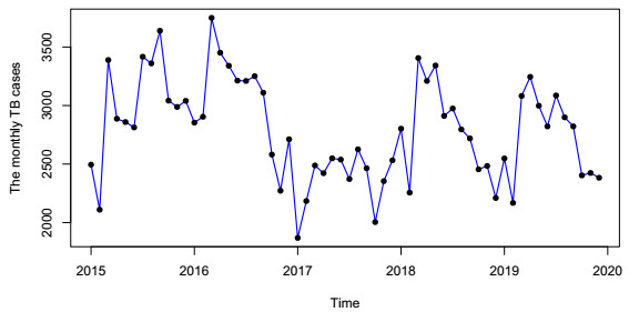
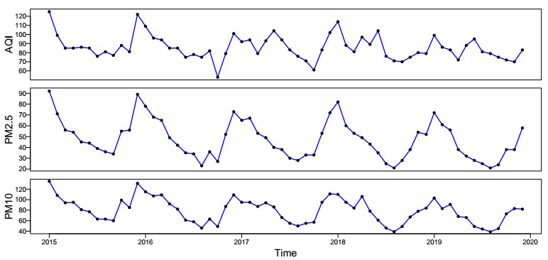
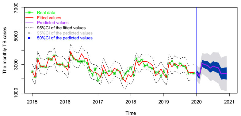
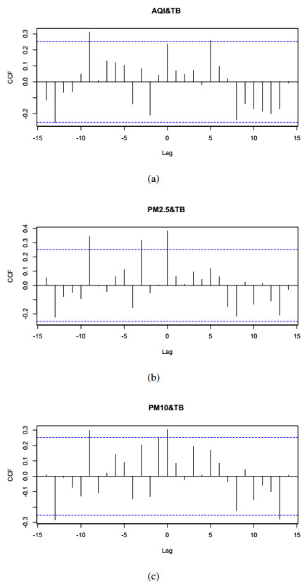
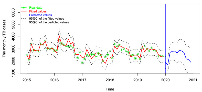
In this paper, we investigate the relationship between the air pollution and tuberculosis cases and its prediction in Jiangsu, China by using the time-series analysis method, and find that the seasonal ARIMA(1, 1, 0)×(0, 1, 1)12 model is the preferred model for predicting the TB cases in Jiangsu, China. Furthermore, we evaluate the relationship between AQI, PM2.5, PM10 and the number of TB cases, and find that the prediction accuracy of the ARIMA model is improved by adding monthly PM2.5 with 0-month lag as an external variable, i.e., ARIMA(1, 1, 0)×(0, 1, 1)12+PM2.5. The results show that ARIMAX model can be a useful tool for predicting TB cases in Jiangsu, China, and it can provide a scientific basis for the prevention and treatment of TB.
Citation: Zuqin Ding, Yaxiao Li, Xiaomeng Wang, Huling Li, Yongli Cai, Bingxian Wang, Kai Wang, Weiming Wang. The impact of air pollution on the transmission of pulmonary tuberculosis[J]. Mathematical Biosciences and Engineering, 2020, 17(4): 4317-4327. doi: 10.3934/mbe.2020238
In this paper, we investigate the relationship between the air pollution and tuberculosis cases and its prediction in Jiangsu, China by using the time-series analysis method, and find that the seasonal ARIMA(1, 1, 0)×(0, 1, 1)12 model is the preferred model for predicting the TB cases in Jiangsu, China. Furthermore, we evaluate the relationship between AQI, PM2.5, PM10 and the number of TB cases, and find that the prediction accuracy of the ARIMA model is improved by adding monthly PM2.5 with 0-month lag as an external variable, i.e., ARIMA(1, 1, 0)×(0, 1, 1)12+PM2.5. The results show that ARIMAX model can be a useful tool for predicting TB cases in Jiangsu, China, and it can provide a scientific basis for the prevention and treatment of TB.

| [1] | WHO, Global tuberculosis report 2018. Geneva: World health organization, 2018. Available from: http://www.who.int/tb/publications/globalreport/en/. |
| [2] | S. Basu, J. R. Andrews, E. M. Poolman, N. R. Gandhi, N. S. Shah, A. Moll, et al., Prevention of nosocomial transmission of extensively drug-resistant tuberculosis in rural south african district hospitals: an epidemiological modelling study, Lancet, 370 (2007), 1500-1507. |
| [3] | S. D. Lawn, A. I. Zumla, Tuberculosis, Lancet, 378 (2011), 57-72. |
| [4] |
B. I. Restrepo, Convergence of the tuberculosis and diabetes epidemics: renewal of old acquaintances, Clin. Infect. Dis., 45 (2007), 436-438. doi: 10.1086/519939

|
| [5] | The reported tuberculosis cases in jiangsu province, 2018. Available from: http://www.jshealth.com/. |
| [6] | B. O. Ekpenyong, ARMA type modeling of certain non-stationary time series in calabar, Am. J. Appl. Math. Stat., 4 (2016), 118-125. |
| [7] | M. Moosazadeh, N. Khanjani, M. Nasehi, A. Bahrampour, Predicting the incidence of smear positive tuberculosis cases in iran using time series analysis, Iran. J. Publ. Health, 44 (2015), 1526-1534. |
| [8] | H. Li, R. Zheng, Q. Zheng, W. Jiang, X. Zhang, W. M. Wang, et al., Predicting the number of visceral leishmaniasis cases in Kashgar, Xinjiang, China using the ARIMA-EGARCH model, Asian Pac. J. Trop. Med., 13 (2020), 81-90. |
| [9] | S. Tang, Q. Yan, W. Shi, X. Wang, X. Sun, P. Yu, et al., Measuring the impact of air pollution on respiratory infection risk in china, Environ. Pollut., 232 (2018), 1-10. |
| [10] | Y. Alyousifi, N. Masseran, K. Ibrahim, Modeling the stochastic dependence of air pollution index data, Stoch. Env. Res. Risk., 26 (2018), 1603-1611. |
| [11] | S. Chauhan, S. Bhatia, S. Gupta, Effect of pollution on dynamics of sir model with treatment, Int. J. Biomath., 8 (2015), 1550083. |
| [12] | M. Laeremans, E. Dons, I. Avila-Palencia, G. Carrasco-Turigas, Short-term effects of physical activity, air pollution and their interaction on the cardiovascular and respiratory system, Environ. Int., 117 (2018), 82-90. |
| [13] |
P. M. Mannucci, Airborne pollution and cardiovascular disease: burden and causes of an epidemic, Eur. Heart. J., 34 (2013), 1251-1253. doi: 10.1093/eurheartj/eht045
|
| [14] |
G. Polezer, Y. Tadano, H. Siqueira, A. Godoi, C. Yamamoto, Assessing the impact of pm 2.5 on respiratory disease using artificial neural networks, Environ. Pollut., 235 (2018), 394-403. doi: 10.1016/j.envpol.2017.12.111
|
| [15] |
C. Sun, Y. Xiang, Y. Xin, Social acceptance towards the air pollution in china: Evidence from public's willingness to pay for smog mitigation, Energy Policy, 92 (2016), 313-324. doi: 10.1016/j.enpol.2016.02.025
|
| [16] |
Z. Peng, C. Liu, B. Xu, H. Kan, W. Wang, Long-term exposure to ambient air pollution and mortality in a chinese tuberculosis cohort, Sci. Total Environ., 580 (2017), 1483-1488. doi: 10.1016/j.scitotenv.2016.12.128
|
| [17] | C. Liu, R. Chen, F. Sera, A. M. Vicedo-Cabrera, Y. Guo, S. Tong, et al., Ambient particulate air pollution and daily mortality in 652 cities, N. Engl. J. Med., 381 (2019), 705-715. |
| [18] | S. He, S. Tang, W. M. Wang, A stochastic SIS model driven by random diffusion of air pollutants, Phys. A, 532 (2019), 121759. |
| [19] |
S. He, S. Tang, Y. Xiao, R. A. Cheke, Stochastic modelling of air pollution impacts on respiratory infection risk, Bull. Math. Biol., 80 (2018), 3127-3153. doi: 10.1007/s11538-018-0512-5
|
| [20] | National meteorological information center. Available from: http://data.cma.cn/. |
| [21] |
S. Chadsuthi, C. Modchang, Y. Lenbury, S. Iamsirithaworn, W. Triampo, Modeling seasonal leptospirosis transmission and its association with rainfall and temperature in Thailand using timeseries and ARIMAX analyses, Asian Pac. J. Trop. Med., 5 (2012), 539-546. doi: 10.1016/S1995-7645(12)60095-9
|
Figures(8) / Tables(5)

Zuqin Ding, Yaxiao Li, Xiaomeng Wang, Huling Li, Yongli Cai, Bingxian Wang, Kai Wang, Weiming Wang. The impact of air pollution on the transmission of pulmonary tuberculosis[J]. Mathematical Biosciences and Engineering, 2020, 17(4): 4317-4327. doi: 10.3934/mbe.2020238


 DownLoad: