Plasma HGF concentration in patients with brain tumors

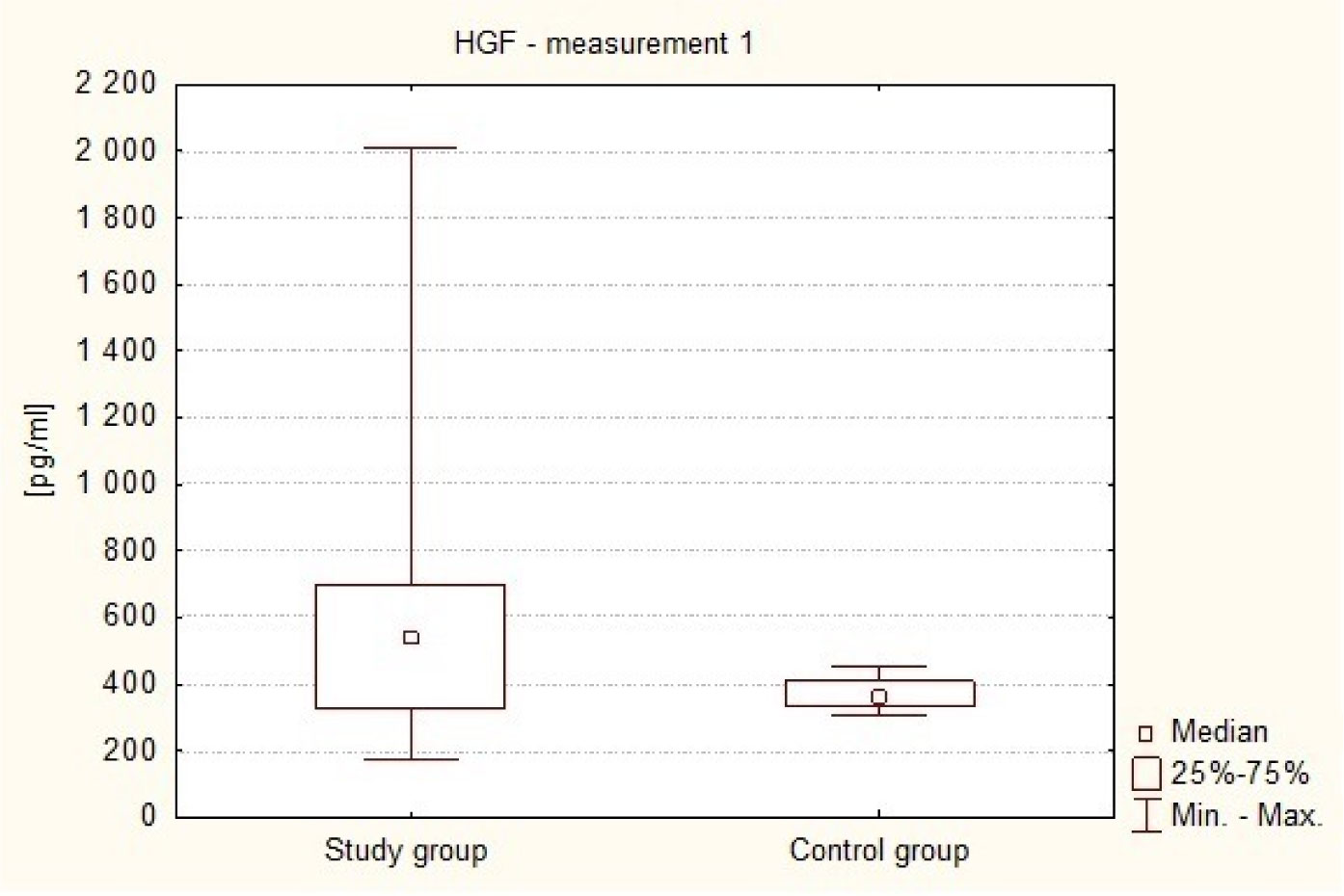
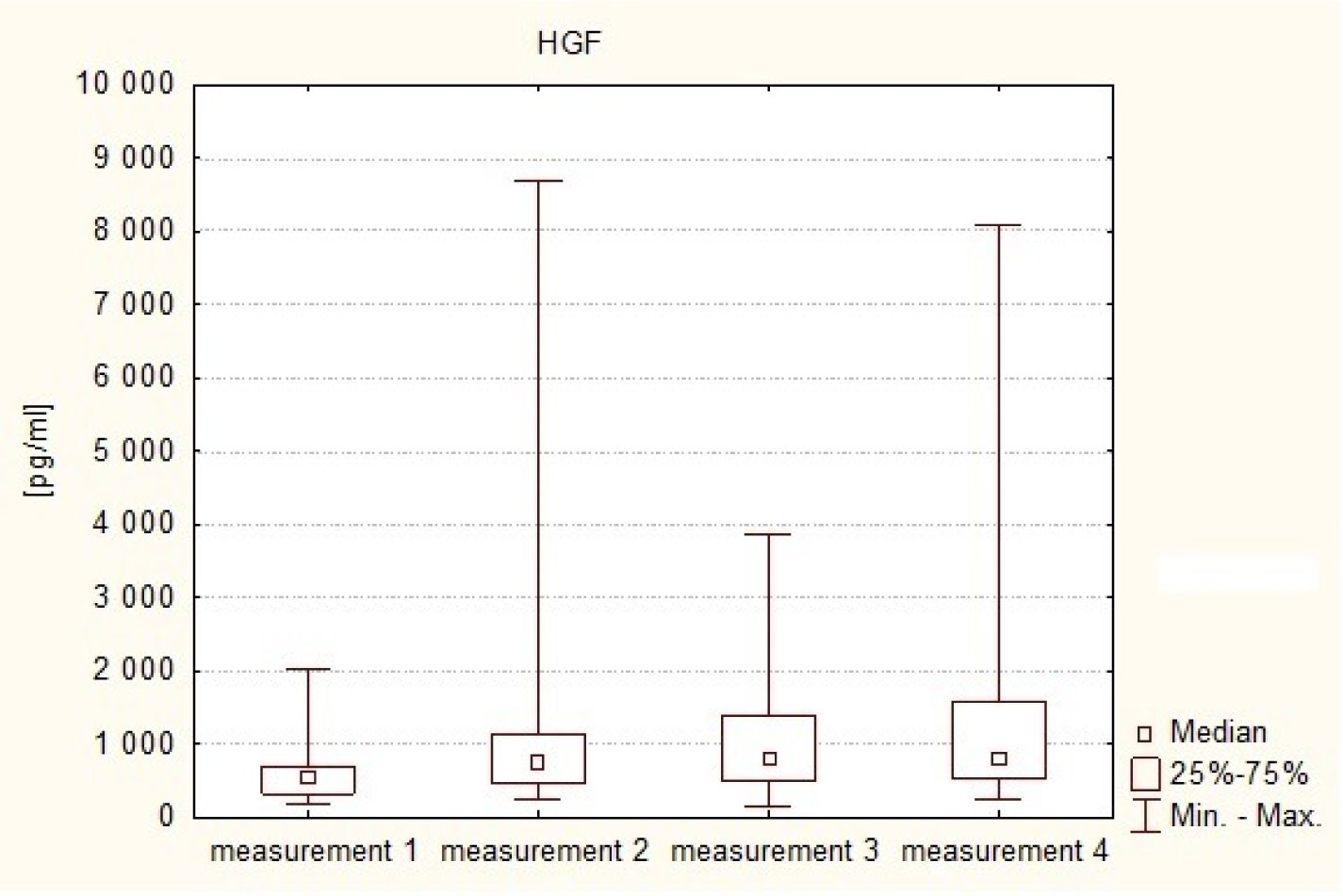
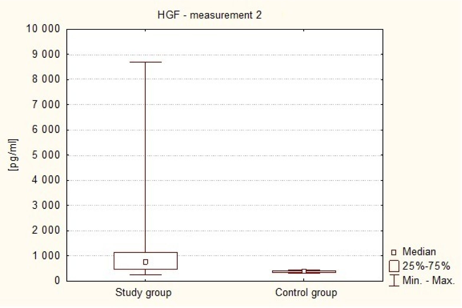
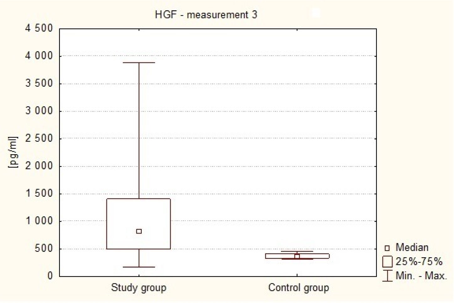
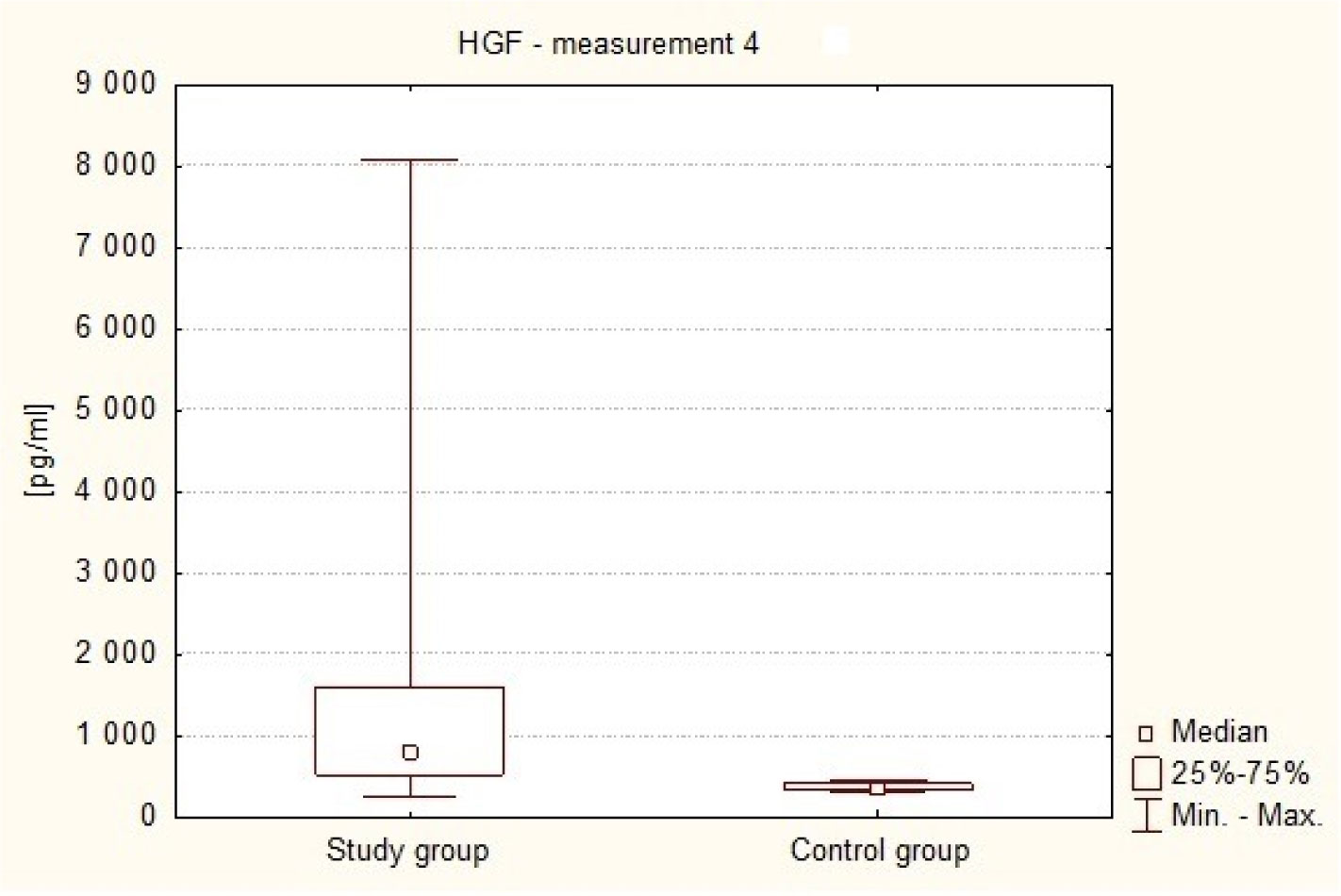
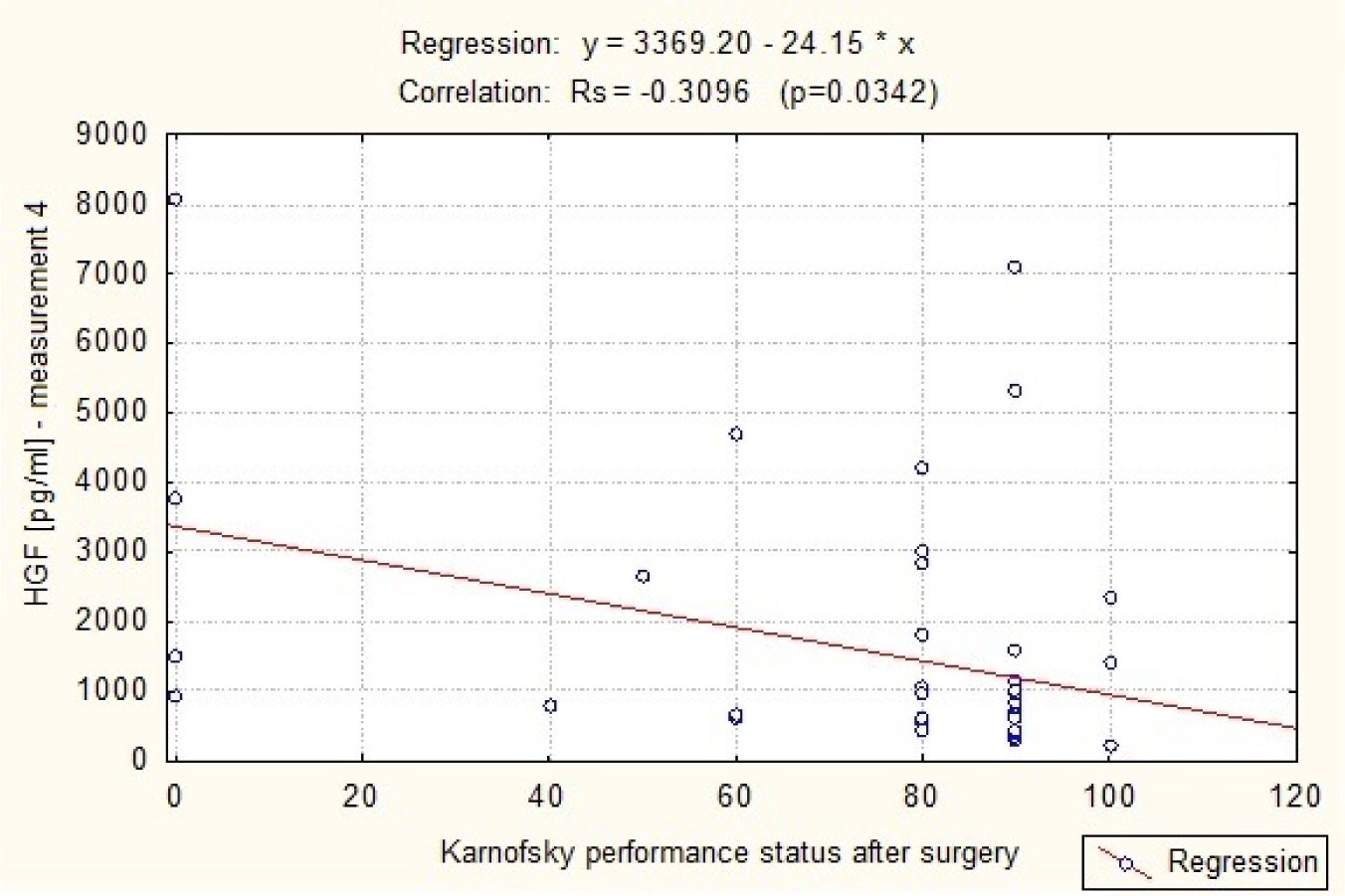
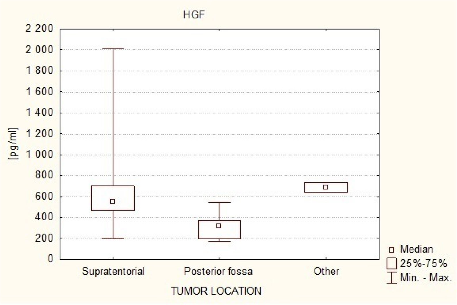
1.   Introduction

The Human Immunodeficiency Virus (HIV) is responsible for a very high number of deaths worldwide. Acquired ImmunoDeficiency Syndrome (AIDS) is a disease of the human immune system caused by infection with HIV. The HIV virus can be transmitted by several ways but there is no cure or vaccine for AIDS. Nevertheless, antiretroviral (ART) treatment improves health, prolongs life and reduces the risk of HIV transmission. The ART treatment increases life expectation but has some limitations. For instance, it doesn't restore health, has some side effects, and is very expensive. Individuals infected with HIV are more likely to develop tuberculosis because of their immunodeficiency, so a model that considers HIV and tuberculosis is very interesting to investigate. One can find many studies in the literature ^[1,2,3]. A TB-HIV/AIDS co-infection model, that contains the celebrated SICA (Susceptible–Infected–Chronic–AIDS) model as a sub-model, was first proposed in ^[4]:

where

with

the total population at time $t$. The meaning of the parameters that appear in the SICA model (1.1)–(1.3) are given in Table 1.

The model considers a varying population size in a homogeneously mixing population, subdividing the human population into four mutually-exclusive compartments:

$-$ susceptible individuals ($S$);

$-$ HIV-infected individuals with no clinical symptoms of AIDS (the virus is living or developing in the individuals but without producing symptoms or only mild ones) but able to transmit HIV to other individuals ($I$);

$-$ HIV-infected individuals under ART treatment (the so called chronic stage) with a viral load remaining low ($C$);

$-$ HIV-infected individuals with AIDS clinical symptoms ($A$).

The SICA model has some assumptions. It can be seen in ^[5] that the susceptible population is increased by the recruitment of individuals into the population, assumed susceptible at a rate $\Lambda$. All individuals suffer from natural death at a constant rate $\mu$. Susceptible individuals $S$ acquire HIV infection, following effective contact with people infected with HIV, at rate $\lambda$ (1.2), where $\beta$ is the effective contact rate for HIV transmission. The modification parameter $\eta_{A} \geq 1$ accounts for the relative infectiousness of individuals with AIDS symptoms, in comparison to those infected with HIV with no AIDS symptoms. Individuals with AIDS symptoms are more infectious than HIV-infected individuals because they have a higher viral load and there is a positive correlation between viral load and infectiousness. On the other hand, $\eta_{C} \leq 1$ translates the partial restoration of the immune function of individuals with HIV infection that use correctly ART. The SICA mathematical model (1.1)–(1.3) is well-studied in the literature ^[5]. It has shown to provide a proper description with respect to the HIV/AIDS situation in Cape Verde ^[6] and recent extensions include stochastic transmission ^[7] and fractional versions with memory and general incidence rates ^[8]. Here our main aim is to propose, for the first time in the literature, a discrete-time SICA model.

For most nonlinear continuous models in engineering and natural sciences, it is not possible to obtain an exact solution ^[9], so a variety of methods have been constructed to compute numerical solutions ^[10,11]. It is well known that numerical methods, like the Euler and Runge–Kutta, among others, often fail to solve nonlinear systems. One of the reasons is that they generate oscillations and unsteady states if the time step size decreases to a critical size ^[12]. Among available approaches to address the problem, the nonstandard finite discrete difference (NSFD) schemes, introduced by Mickens in ^[13,14], have been successfully applied to several different epidemiological models ^[15,16]. Precisely, the NSFD schemes were created to eliminate or reduce the occurrence of numerical instabilities that generally arise while using other methods. This is possible because there are some designed laws that systems must satisfy in order to preserve the qualitative properties of the continuous model, such as positivity, boundedness, stability of the equilibrium points, conservation laws, and others ^[17]. The literature on Mickens-type NSFD schemes is now vast ^[18,19]. The paper ^[20] considers the NSFD method of Mickens and apply it to a dynamical system that models the Ebola virus disease. In ^[21], a NSFD scheme is designed in which the Metzler matrix structure of the continuous model is carefully incorporated and both Mickens' rules on the denominator of the discrete derivative and the nonlocal approximation of nonlinear terms are used. In that work the general analysis is detailed for a MSEIR model. In ^[22], the authors summarize NSFD methods and compare their performance for various step-sizes when applied to a specific two-sex (male/female) epidemic model; while in ^[23] it is shown that Mickens' approach is qualitatively superior to the standard approach in constructing numerical methods with respect to productive-destructive systems (PDS's). NSFD schemes for PDS's are also investigated in ^[24]; NSFD methods for predator-prey models with the Beddington–De Angelis functional response are studied in ^[25]. Here we propose and investigate, for the first time in the literature, the dynamics of a discretized SICA model using the Mickens NSFD scheme.

The paper is organized as follows. Some considerations, regarding the continuous SICA model and the stability of discrete-time systems, are presented in section 2. The original results are then given in section 3: we start by introducing the discretized SICA model; we find the equilibrium points, prove the positivity, Theorem 3, and boundedness of the solutions, Theorem 4; we also establish the local stability of the disease free equilibrium point of the discrete model, Theorem 5, as well as the global stability of the equilibrium points, Theorems 6 and 7. In section 4, we provide some numerical simulations to illustrate the stability of the NSFD discrete SICA model using a case study. We end with section 5 of conclusion.

2.   Preliminaries

In this section, we collect some preliminary results about the continuous SICA model ^[4], as well as results for the stability of discrete-time systems ^[26], useful in our work.

2.1.   The continuous SICA model

All the information in this section is proved in ^[4]. Each solution $(S(t), I(t), C(t), A(t))$ of the continuous model much satisfy $S(0) \geq 0$, $I(0) \geq 0$, $C(0) \geq 0$, and $A(0) \geq 0$, because each equation represents groups of human beings. Adding the four equations of (1.1), one has

so that

Therefore, the biologically feasible region is given by

which is positively invariant and compact. This means that it is sufficient to study the qualitative dynamics in $\Omega$. The model has two equilibrium points: a disease free and an endemic one. The disease free equilibrium (DFE) point is given by

Following the approach of the next generation matrix ^[27], the basic reproduction number $R_{0}$ for model (1.1), which represents the expected average number of new infections produced by a single HIV-infected individual in contact with a completely susceptible population, is given by

where along all the manuscript we use $C_{1} = \rho + \phi + \mu$, $C_{2} = \alpha + \mu+ d$, and $C_{3} = \omega + \mu$. The endemic point has the following expression:

where $D = -(\lambda^{\ast} +\mu) (\mu (C_{3}(\rho + C_{2}) +C_{2} \phi + \rho d) + \rho \omega d)$ and

which is positive if $\mathcal{R}_{0} > 1$. The explicit expression of the endemic equilibrium point of (1.1) is given by

Regarding the stability of the equilibrium points, Theorem 3.1 and Proposition 3.4 of ^[4] establish the persistence of the endemic point. The disease is persistent in the population if the infected cases with AIDS are bounded away from zero or the population $S$ disappears. The local stability of the endemic point is given in Theorem 3.8 of ^[4]. Lemma 3.5 of ^[4] states that the DFE is locally asymptotically stable if $R_{0} < 1$ and unstable if $R_{0} > 1$. Finally, Theorem 3.6 of ^[4] asserts that, under suitable conditions, the DFE point is globally asymptotically stable. Here we prove similar properties in the discrete-time setting (section 3). For that we now recall an important tool for difference equations.

2.2.   The Schur–Cohn criterion

One of the main tools that provides necessary and sufficient conditions for the zeros of a $n$th-degree polynomial

to lie inside the unit disk is the Schur–Cohn criterion ^[26]. This result is useful for studying the stability of the zero solution of a $k$th-order difference equation or to investigate the stability of a $k$-dimensional system of the form

where $p(\lambda)$ in (2.3) is the characteristic polynomial of the matrix $A$. Let us introduce some preliminaries before presenting the Schur–Cohn criterion. Namely, let us define the inners of a matrix $B = (b_{ij})$. The inners of a matrix are the matrix itself and all the matrices obtained by omitting successively the first and last columns and first and last rows. A matrix $B$ is said to be positive innerwise if the determinant of all its inners are positive.

Theorem 1 (The Shur–Cohn criterion ^[26]). The zeros of the characteristic polynomial (2.3) lie inside the unit disk if, and only if, the following holds:

i) $p(1) > 0$;

ii) $(-1)^{k}p(-1) > 0$;

iii) the $(k-1) \times (k-1)$ matrices

are positive innerwise.

Using the Schur–Cohn criterion, one may obtain necessary and sufficient conditions on the $p_{i}$ coefficients such that the zero solution of (2.3) is locally asymptotically stable.

Theorem 2 (See ^[26]). Let $A \in \mathcal{M}_{k \times k}$ and let (2.3) be its characteristic polynomial. Then, $p(\lambda)$ is a polynomial of degree $k$. Moreover, $p(\lambda)$ has the form

3.   Main results

We begin by proposing a discrete-time SICA model.

3.1.   The NSFD scheme

One of the important features of the discrete-time epidemic models obtained by Mickens method is that they present the same features as the corresponding original continuous-time models. Here, we construct a dynamically consistent numerical NSFD scheme for solving (1.1) based on ^[13,14,17]. Let us define the time instants $t_{n} = nh$ with $n$ integer, $h = t_{n+1} -t_{n}$ as the time step size, and $(S_{n}, I_{n}, C_{n}, A_{n})$ as the approximated values of $(S(nh), I(nh), C(nh), A(nh))$. Thus, the NSFD scheme for model (1.1) takes the following form:

where $\tilde{\lambda}_{n} = \frac{\beta}{N_{n}}(I_{n}+\eta_{C}C_{n}+\eta_{A}A_{n})$. The nonstandard schemes are based in two fundamental principles ^[14,17]:

1. Regarding the first derivative, we have

where $\nu(h)$ and $\psi(h)$ are the numerator and denominator functions that satisfy the requirements

In general, the numerator function can be selected to be $\nu(h) = 1$. We will make this choice here. Generally, the denominator function is nontrivial. Based on Mickens work ^[28,29], when we write explicitly $S_{n+1}$ using $\phi(h) = h$, we have in the denominator the term $1+\mu h$, which means that we can use $\psi(h) = \dfrac{{{\rm{e}}}^{\mu h}-1}{\mu}$ as the denominator function. Throughout our study, $\psi(h) = \dfrac{{{\rm{e}}}^{\mu h}-1}{\mu}$ but, for brevity, we write $\psi(h) = \psi$.

2. Both linear and nonlinear functions of $x(t)$ and its derivatives may require a "nonlocal" discretization. For example, $x^{2}$ can be replaced by $x_{k} x_{k+1}$.

Since model (3.1) is linear in $S_{n+1}$, $I_{n+1}$, $C_{n+1}$, and $A_{n+1}$, we can obtain their explicit form:

3.2.   Positivity of solutions

The first result to be shown is the positivity of the solutions.

Theorem 3. If all the initial and parameter values of the discrete system (3.2) are positive, then the solutions are always positive for all $n \geq 0$ with denominator function $\psi$.

Proof. Let us assume that $S(0), I(0), C(0), A(0)$ are positive. We only need to show that $I_{n+1}$ is positive. The denominator is given by

which can be rewritten as

and, simplifying, we get

Since all parameter values are positive, $(S_{n+1}, I_{n+1}, C_{n+1}, A_{n+1})$ is positive for all $n \geq 0$.

3.3.   Conservation law

The second result to be shown is the conservation law or boundedness of the solutions.

Theorem 4. The NSFD scheme defines the discrete dynamical system (3.2) on

Proof. Let the total population be $N_{n} = S_{n}+I_{n}+C_{n}+A_{n}$. Adding the four equations of (3.1), we have

and

By the discrete Grownwall inequality, if $0 < N(0) < \frac{\Lambda}{\mu}$, then

and, since $\left(\dfrac{1}{1+ \mu \psi}\right) < 1$, we have $N_{n} \to \frac{\Lambda}{\mu}$ as $n \to \infty$. We conclude that the feasible region $\tilde{\Omega}$ is maintained within the discrete scheme.

3.4.   Elementary stability

A difference scheme that approximates a first-order differential system is elementary stable if, for any value of the step size, its fixed-points are exactly those of the differential system. Furthermore, when applied to the associated linearized differential system, the resulting difference scheme has the same stability/instability properties ^[30].

The continuous and discrete system have the same equilibria. The disease free equilibrium (DFE) point is given by

The explicit expression of the endemic equilibrium point of (3.2) can be rewritten as the one of the continuous case: when

we obtain the endemic equilibrium point. The explicit expression of the endemic equilibrium point of (3.2) can be rewritten as the one of the continuous case:

After some computations, we get the following equalities:

3.4.1.   Local stability of the DFE point

Let us discuss the stability of the proposed NSFD scheme at the DFE point $E_{0}$ (3.6).

Remark 1. Several articles use the next-generation matrix approach presented in ^[31]. For that, however, the matrices $F+T$ must be non-negative. Our model does not satisfy such condition.

The following technical lemma has an important role in our proofs.

Lemma 1. If $\mathcal{R}_{0} < 1$, then $\beta$ must be smaller than $C_{1}$.

Proof. If $\mathcal{R}_{0} < 1$, then

Since $C_{2}$ and $C_{3}$ are positive, we conclude that $\beta-C_{1} < 0$.

Proposition 1. The first condition of Theorem 1, $p_{4}(1) > 0$, is satisfied if $\mathcal{R}_{0} < 1$.

Proof. The linearization of (3.2) at the DFE $E_{0}$ is:

The characteristic polynomial of $J(E_{0})$ has the following expression:

where $p_{3}(\lambda)$ is given by

that is,

Since $p_{4}(1) > 0$, we have $(-\mu -1)p_{3}(1) > 0$, and recalling that $\mu > 0$, we conclude that

is negative: $p_{3}(1) < 0$. If $\mathcal{R}_{0} < 1$, then

and

Therefore,

and

We conclude that the first condition of Theorem 1 is satisfied if $\mathcal{R}_{0} < 1$.

Proposition 2. If $\mathcal{R}_{0} < 1$, $C_{2} < 1$, $C_{3} < 1$ and $\beta < \frac{C_{2} C_{3}}{(1-C_{2})(1-C_{3})}$, then the second condition of Theorem 1, that is, $(-1)^{4}p_{4}(-1) > 0$, is satisfied.

Proof. Since $(-1)^{4} \cdot p_{4}(-1) > 0$, we have $(-\mu +1)p_{3}(-1) > 0$ and $\mu < 1$, so $p_{3}(-1) > 0$. It can be seen that

If $\mathcal{R}_{0} < 1$, then

and

Thus,

and

We conclude that if $C_{2} < 1$, $C_{3} < 1$, and $\beta < \frac{C_{2} C_{3}}{(1-C_{2})(1-C_{3})}$ are satisfied, then $p_{3}(-1) > 0$.

Proposition 3. If $\mathcal{R}_{0} < 1$, $\mu < \dfrac{1}{\mathcal{D}(1-\mathcal{R}_{0})}$, $p_{2} < 1+p_{4}$, and

then the third condition of Theorem 1 is satisfied.

Proof. The third condition of Theorem 1 is the following: the $3 \times 3$ matrices $B_{3}^{\pm}$ given by

are positive innerwise. Recall that $p_{4}(\lambda) = \lambda^{4}+p_{1}\lambda^{3} +p_{2} \lambda^{2}+p_{3}\lambda +p_{4} = (-\mu-\lambda)p_{3}(\lambda)$ and

or

Also, if $\mathcal{R}_{0} < 1$, then, by Lemma 1, $\beta < C_{1}$. Therefore, $p_{1} > 0$. If we also consider (3.8), and apply it to $p_{2}$ and $p_{3}$, we get

and

In other words, $B_{3}^{+}$ and $B_{3}^{-}$ have the following form:

and their inners must be positive:

1. Regarding $B_{3}^{+}$, we must have

a) $1+p_{4} > 0$;

b) $|B_{3}^{+}| = (1+p_{4})(1+p_{2})-p_{3}(p_{1} +p_{3})+p_{4}(p_{1} (p_{1}+p_{3})-(1+p_{4})(p_{2}+p_{4})) > 0$.

2. Regarding $B_{3}^{-}$, we must have

a) $1-p_{4} > 0$;

b) $|B_{3}^{-}| = (1-p_{4})(1-p_{2})+p_{3}(p_{1}-p_{3}) -p_{4}(p_{1} (p_{1}-p_{3})-(1-p_{4})(p_{2}-p_{4})) > 0$.

Note that $p_{4} = \mu\mathcal{D}(1-\mathcal{R}_{0}) = \det(J(E_{0}))$ and, if $\mathcal{R}_{0} < 1$, then $p_{4} > 0$. Therefore, 1 a) is satisfied. For 2 a) to be satisfied, it is necessary that

Considering 1 b) and 2 b), after some computations, we can rewrite them as

Thus, from (3.12), $p_{2} < 1+p_{4}$, and (3.9), the third condition of Theorem 1 is satisfied.

We are now in condition to prove the main result of this section.

Theorem 5. If $C_{2} < 1$, $C_{3} < 1$, $\beta < \frac{C_{2} C_{3}}{(1-C_{2})(1-C_{3})}$, $p_{2} < 1+p_{4}$, and (3.9) and (3.12) are satisfied, then, provided $\mathcal{R}_{0} < 1$, the disease free equilibrium point of the discrete system (3.2) is locally asymptotically stable. If the previous conditions are not satisfied, then the disease free equilibrium point is unstable.

Proof. The result follows by Theorem 1 and Propositions 1, 2 and 3. If any of the conditions enumerated are not satisfied, at least one of the roots of the characteristic polynomial lies outside the unit circle, so the disease free equilibrium point is unstable.

3.4.2.   Global stability of the equilibrium points

Now we prove that $\mathcal{R}_{0}$ is a critical value for global stability: when $\mathcal{R}_{0} < 1$, the disease free equilibrium point is globally asymptotically stable; when $\mathcal{R}_{0} > 1$, the endemic equilibrium is globally asymptotically stable.

Theorem 6. If $\mathcal{R}_{0} < 1$, then the DFE point of the discrete-time SICA model (3.1) is globally asymptotically stable.

Proof. For any $\varepsilon > 0$, there exists an integer $n_{0}$ such that, for any $n\geq n_{0}$, $S_{n+1} < \frac{\Lambda}{\mu}+ \varepsilon$. Consider the sequence $\{ V(n)\}_{n = 0}^{+ \infty}$ defined by

For any $n \geq n_{0}$,

Since

we have

If $\mathcal{R}_{0} < 1$, and because $\varepsilon$ is arbitrary, we conclude that $V(n+1)-V(n) \leq 0$ and $\underset{n\to \infty}{\lim} I_{n} = 0$ for any $n \geq 0$. The sequence $\{ V(n)\}_{n = 0}^{+ \infty}$ is monotone decreasing and $\underset{n\to \infty}{\lim} S_{n} = \frac{\Lambda}{\mu}$.

Theorem 7. If $\mathcal{R}_{0} > 1$, then the endemic equilibrium point of the discrete-time SICA model (3.1) is globally asymptotically stable.

Proof. We construct a sequence $\{ \tilde{V}(n)\}_{n = 1}^{+\infty}$ of the form

where $g(x) = x-1-\ln(x)$, $x \in \mathbb{R}^{+}$. Clearly, $g(x)\geq 0$ with equality holding true only if $x = 1$. We have

Similarly,

The difference of $\tilde{V}(n)$ satisfies

Therefore, $\{ \tilde{V}(n)\}_{n = 1}^{+\infty}$ is a monotone decreasing sequence for any $n \geq 0$. Since $\tilde{V}(n) \geq 0$ and $\underset{n \to \infty}{\lim}\left(\tilde{V}(n+1) -\tilde{V}(n)\right) = 0$, we obtain that $\underset{n \to \infty}{\lim} S_{n+1} = S^{\ast}$, $\underset{n \to \infty}{\lim} I_{n+1} = I^{\ast}$, $\underset{n \to \infty}{\lim} C_{n+1} = C^{\ast}$ and $\underset{n \to \infty}{\lim} A_{n+1} = A^{\ast}$. This completes the proof.

4.   Numerical simulations

In this section, we apply our discrete model to a case study of Cape Verde ^[5,6]. The data is the same of ^[5] and the parameters too. We present here a resume of the information.

Since the first diagnosis of AIDS in 1986, Cape Verde try to fight, prevent, and treat HIV/AIDS ^[6,32]. In Table 2, the cumulative cases of infection by HIV and AIDS in Cape Verde from 1987 to 2014 is given. Based on ^[32,33], the values for the initial conditions are taken as

Regarding the parameter values, we consider $\rho = 0.1$ ^[34] and $\gamma = 0.33$ ^[35]. It is assumed that, after one year, HIV infected individuals, $I$, that are under ART treatment, have low viral load ^[36] and are transferred to class $C$, so that $\phi = 1$. The ART treatment therapy takes a few years. Following ^[6], it is assumed the default treatment rate to be 11 years ($1 / \omega$ years, to be precise). Based in ^[37], the induced death rate by AIDS is $d = 1$. From the World Bank data ^[33,38], the natural rate is assumed to be $\mu = 1/69.54$. The recruitment rate $\Lambda = 13045$ was estimated in order to approximate the values of the total population of Cape Verde, see Table 2. Based on a research study known as HPTN 052, where it was found that the risk of HIV transmission among heterosexual serodiscordant is $96\%$ lower when the HIV-positive partner is on treatment ^[39], we take here $\eta_{C} = 0.04$, which means that HIV infected individuals under ART treatment have a very low probability of transmitting HIV ^[40]. For the parameter $\eta_{A} \geq 1$, which accounts the relative infectiousness of individuals with AIDS symptoms, in comparison to those infected with HIV with no AIDS symptoms, we assume, based on ^[41], that $\eta_{A} = 1.35$. For $(\eta_{C}, \eta_{A}) = (0.04, 1.35)$, the estimated value of the HIV transmission rate is equal to $\beta = 0.695$. Using these parameter values, the basic reproduction number is $\mathcal{R}_{0} = 4.5304$ and the endemic equilibrium point $(S^{\ast}, I^{\ast}, C^{\ast}, A^{\ast}) = (145276, 48136.4, 461146, 3580.57)$. In Figure 1, we show graphically the cumulative cases of infection by HIV/AIDS in Cape Verde given in Table 2, together with the curves obtained from the continuous-time SICA model (1.1) and our discrete-time SICA model (3.1). Our simulations of the continuous and discrete models were done with the help of the software Wolfram $\textsf{Mathematica}$, version 12.1. For the continuous model, we have used the command $\texttt{NSolve}$, that computes the solution by interpolation functions. Our implementation for the discrete case makes use of the $\textsf{Mathematica}$ command $\texttt{RecurrenceTable}$.

To illustrate the global stability of the endemic equilibrium (EE), predicted by our Theorem 7, we consider different initial conditions borrowed from ^[5], from different regions of the plane:

The obtained results are given in Figure 2.

5.   Conclusions

In this work, we proposed a discrete-time SICA model, using Mickens' nonstandard finite difference (NSFD) scheme. The elementary stability was studied and the global stability of the equilibrium points proved. Finally, we made some numerical simulations, comparing our discrete model with the continuous one. For that, we have used the same data, following the case study of Cape Verde. Our conclusion is that the discrete model can be used with success to describe the reality of Cape Verde, as well as to properly approximate the continuous model. All our simulations have been done using the numerical computing environment Mathematica, version 12.1, running on an Apple MacBook Pro i5 2.5 GHz with 16Gb of RAM. The solutions of the models were found in "real time".

Mickens was a pioneer in NSFD schemes. Throughout the years, other NSFD schemes were developed. Roughly speaking, different Mickens-type methods differ on the denominator functions and the discretization, depending on concrete conditions that the continuous model under study must satisfy. In ^[20], the incidence rate is combined, while in ^[21] all parameters are constant. Other types of NSFD are presented, e.g., in ^{[22,23,24,25]}, which can be used if the system satisfy some conditions and a suitable denominator function is constructed. For such schemes, the incidence functions are different from ours. In ^[23], for example, it is fundamental to rewrite the system and the discretization method and the denominator function are different from the ones we use here. The article ^[24] uses the same approach of ^[23] and the model has a bilinear incidence function. Positive and elementary stable nonstandard finite-difference methods are also considered in ^[25]. Mickens set the field, but several different authors developed and are developing other related discretization methods. For the SICA model, however, as we have shown, a new NSFD scheme is not necessary and the standard Mickens' method provides a well posed discrete-time model with excellent results, without the need to impose additional conditions to the model.

Acknowledgments

The authors were partially supported by the Portuguese Foundation for Science and Technology (FCT): Sandra Vaz through the Center of Mathematics and Applications of Universidade da Beira Interior (CMA-UBI), project UIDB/00212/2020; Delfim F. M. Torres through the Center for Research and Development in Mathematics and Applications (CIDMA), project UIDB/04106/2020. They are very grateful to three anonymous referees, who kindly reviewed an earlier version of this manuscript and provided valuable suggestions and comments.

Conflict of interest

The authors declare that they have no conflicts of interest.